GROUP BY, But for Pixels

Many raster analyses need one result for each polygon. Examples include mean elevation by canton, forest cover by district, and flood depth by parcel. A raster stores values in a grid of pixels. A polygon defines an area, also called a zone.

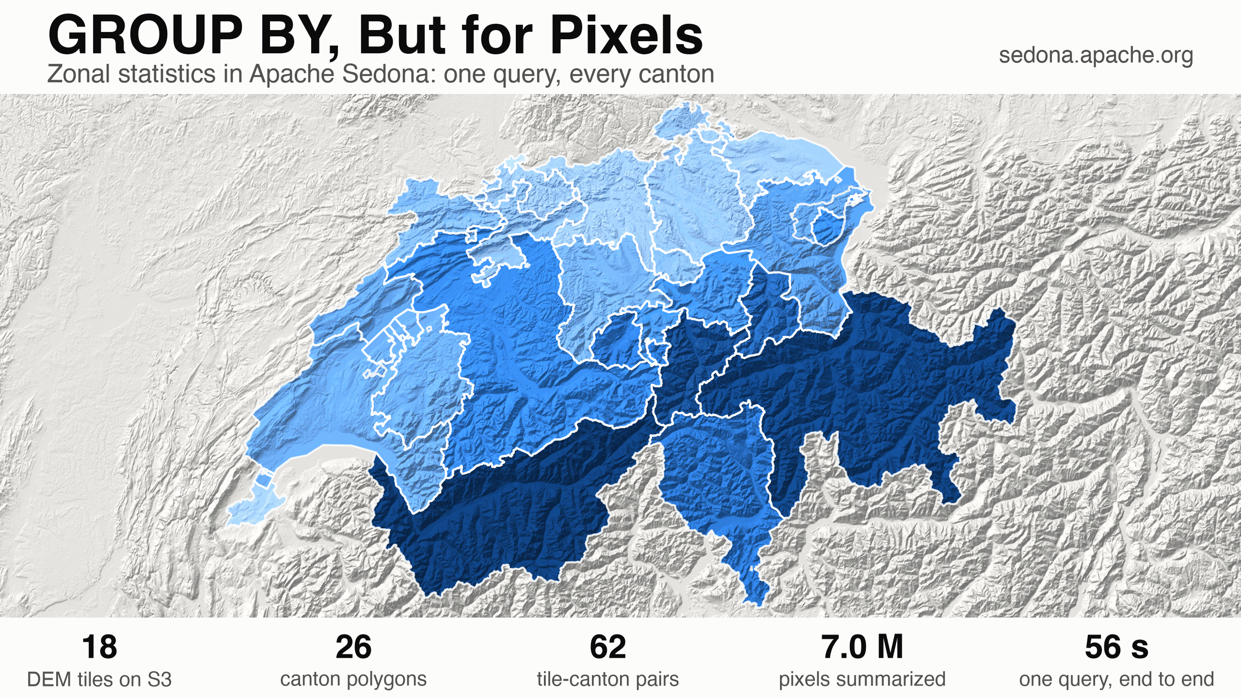
Zonal statistics summarize the raster pixels inside each zone. A spatial join matches data by location. Apache Sedona performs both steps in one query. This example reads 7,006,027 elevation pixels from Amazon S3 and summarizes all 26 Swiss cantons in 56 seconds.

One call, nine numbers

RS_ZonalStatsAll(raster, zone) calculates nine statistics for the raster pixels inside a geometry. It returns a struct with these named fields: count, sum, mean, median, mode, stddev, variance, min, and max. A struct is one value that contains several named fields. The mean is the arithmetic average. Use RS_ZonalStats(raster, zone, 'mean') when one statistic is enough.

By default, Sedona includes a pixel when its center is inside the zone. This rule works well for large zones. For a zone that is only a few pixels wide, pass allTouched = true to include every pixel that the geometry touches.

RS_ZonalStatsAll excludes NODATA pixels by default. NODATA marks a pixel that has no valid measurement. If a zone contains NODATA pixels, its mean uses the remaining valid pixels.

Sedona also checks the coordinate reference system, or CRS. A CRS defines how coordinates map to locations on Earth. If the zone and raster use different systems, Sedona converts the zone to the raster's CRS before it calculates the statistics.

Switzerland in one query

The elevation data comes from the Copernicus 90 m DEM. A digital elevation model, or DEM, stores ground height in a raster. This public dataset stores one GeoTIFF raster file for each 1° tile. Eighteen files cover Switzerland.

The tiled raster reader from our post about the 2 GB limit reads the files from S3. The option retile = false keeps each file in one row:

dem = (
    sedona.read.format("raster")
    .option("retile", "false")
    .load(
        "s3a://copernicus-dem-90m/"
        "Copernicus_DSM_COG_30_N4{5,6,7}_00_E0{05,06,07,08,09,10}_00_DEM/*_DEM.tif"
    )
)
dem.createOrReplaceTempView("dem")

Each row contains 1,200 × 1,200 pixels. The data uses EPSG:4326, a geographic CRS, with a pixel size of 3 arc-seconds. The 26 Swiss cantons are the zones. Sedona reads their polygons from the Overture divisions dataset. The files use GeoParquet, a format for geographic data.

Session setup and canton data

from sedona.spark import SedonaContext

config = (
    SedonaContext.builder()
    .master("local[4]")
    .config("spark.driver.memory", "10g")
    .config(
        "spark.jars.packages",
        "org.apache.sedona:sedona-spark-shaded-3.5_2.12:1.9.1,"
        "org.datasyslab:geotools-wrapper:1.9.1-33.5,"
        "org.apache.hadoop:hadoop-aws:3.3.4",
    )
    .config(
        "spark.hadoop.fs.s3a.aws.credentials.provider",
        "org.apache.hadoop.fs.s3a.AnonymousAWSCredentialsProvider",
    )
    .config(
        "spark.hadoop.fs.s3a.bucket.copernicus-dem-90m.endpoint.region", "eu-central-1"
    )
    .getOrCreate()
)
sedona = SedonaContext.create(config)

cantons = (
    sedona.read.format("geoparquet")
    .load(
        "s3a://overturemaps-us-west-2/release/2026-08-19.0/"
        "theme=divisions/type=division_area/"
    )
    .where("bbox.xmin BETWEEN 5.5 AND 10.7 AND bbox.ymin BETWEEN 45.7 AND 47.9")
    .where("country = 'CH' AND subtype = 'region'")
    .selectExpr("names.primary AS name", "geometry")
)
cantons.createOrReplaceTempView("cantons")

This SQL query joins the raster tiles to the cantons and calculates the results:

WITH parts AS (
    SELECT c.name, RS_ZonalStatsAll(d.rast, c.geometry) AS s
    FROM dem d JOIN cantons c ON RS_Intersects(d.rast, c.geometry)
)
SELECT name,
       ROUND(SUM(s.sum) / SUM(s.count)) AS mean_m,
       ROUND(MIN(s.min)) AS min_m,
       ROUND(MAX(s.max)) AS max_m
FROM parts
WHERE s.count > 0
GROUP BY name
ORDER BY mean_m DESC

The query returns 26 rows and summarizes 7,006,027 pixels. The first run has no cached data and takes 56 seconds. Cantons in the Alps appear at the top of the table:

+----------------------------+---------+------+-----+------+
|name                        |px       |mean_m|min_m|max_m |
+----------------------------+---------+------+-----+------+
|Valais/Wallis               |876887.0 |2138.0|368.0|4534.0|
|Graubünden/Grischun/Grigioni|1202449.0|2023.0|256.0|3961.0|
|Uri                         |182555.0 |1901.0|433.0|3579.0|
|Glarus                      |116676.0 |1584.0|411.0|3597.0|
|Ticino                      |472768.0 |1400.0|193.0|3360.0|
|Obwalden                    |83282.0  |1342.0|433.0|3172.0|
|Bern/Berne                  |1008137.0|1202.0|402.0|4082.0|
|Appenzell Innerrhoden       |29553.0  |1133.0|571.0|2431.0|
+----------------------------+---------+------+-----+------+

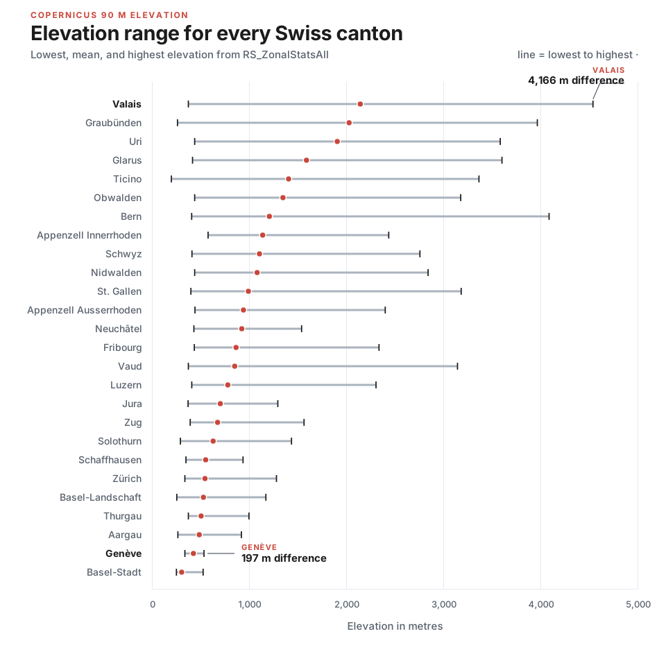
The difference between the lowest and highest point is 4,166 m in Valais. The difference is 197 m in Genève. Both results come from the same query.

Why one canton can produce several rows

RS_Intersects(d.rast, c.geometry) joins each raster tile to every canton that overlaps it. This is a raster-vector spatial join: one side contains raster tiles, and the other contains polygon shapes. The 26 cantons and 18 tiles produce 62 matching pairs. A canton that crosses a tile boundary has one result for each tile.

Genève crosses the 6°E tile boundary, so it produces two rows:

+------+--------+--------+----------------------------------------------------------------------------------------------------------------------------------------------+
|name  |tile_lon|tile_lat|s                                                                                                                                             |
+------+--------+--------+----------------------------------------------------------------------------------------------------------------------------------------------+
|Genève|5.0     |47.0    |{2761.0, 1133564.8060302734, 410.5631314850678, 411.58612060546875, 345.5, 41.7174495306343, 1740.3455953410198, 332.0, 515.2003784179688}    |
|Genève|6.0     |47.0    |{44656.0, 1.8780723717163086E7, 420.56439710594384, 423.7024383544922, 368.0, 34.66281959027446, 1201.5110619479146, 346.5, 529.1962280273438}|
+------+--------+--------+----------------------------------------------------------------------------------------------------------------------------------------------+

Each tile and canton pair is a separate unit of work. Spark can process the 62 pairs in parallel. The same SQL pattern also works with more tiles and zones. Spark sends the pairs to worker processes across the cluster. The driver manages the query, but it does not receive the raster tiles.

How to combine results from several tiles

When a canton overlaps several tiles, the final GROUP BY must combine the partial results. Each statistic needs the correct formula:

• Add count and sum. Addition works for any number of pairs.
• Combine min and max by taking the lowest minimum and the highest maximum.
• Calculate mean as a ratio: SUM(s.sum) / SUM(s.count). Do not average the mean from each pair. That method gives the same weight to 2,761 pixels and 44,656 pixels, which changes Genève's result by 5 m.
• Do not combine median, mode, stddev, or variance from the partial values. For example, the median of several tile medians is not the median of all pixels. These statistics need all pixels for the zone in one raster row. retile = false is enough when the zone fits inside one source raster. Otherwise, merge the tiles with RS_Union_Aggr before the zonal statistics call.

One more case can produce a wrong number without an error. RS_Intersects compares the tile boundary with the zone. A tile can overlap a zone even when no pixel center is inside it. One of the 62 pairs has this result, and RS_ZonalStatsAll returns nine zeros:

+----------------------------+---------------------------------------------+
|name                        |s                                            |
+----------------------------+---------------------------------------------+
|Graubünden/Grischun/Grigioni|{0.0, 0.0, 0.0, 0.0, 0.0, 0.0, 0.0, 0.0, 0.0}|
+----------------------------+---------------------------------------------+

One of those zeros is the min value. If that row enters MIN(s.min), the result for Graubünden becomes 0 m:

+----------------------------+---------+------------+
|name                        |naive_min|filtered_min|
+----------------------------+---------+------------+
|Graubünden/Grischun/Grigioni|0.0      |255.5       |
+----------------------------+---------+------------+

The filter WHERE s.count > 0 removes empty pairs. The correct minimum for Graubünden is 255.5 m. Apply this filter before the final GROUP BY.

Use the same pairs for another question

Zonal statistics can process a raster that a query creates. This example starts with the elevation DEM. A Python user-defined function, or UDF, uses NumPy to calculate the slope of each pixel. The UDF returns the slope values as a new raster column:

@udf(returnType=RasterType())
def slope_deg(raster):
    z = raster.as_numpy_masked()[0].astype(np.float64)
    t = raster.affine_trans
    lat = t.ip_y + t.scale_y * raster.height / 2.0
    m_per_deg_x = 111320.0 * math.cos(math.radians(lat))
    dzdy, dzdx = np.gradient(z, abs(t.scale_y) * 111320.0, abs(t.scale_x) * m_per_deg_x)
    slope = np.degrees(np.arctan(np.hypot(dzdx, dzdy)))
    out = np.where(np.isnan(slope), -9999.0, slope).astype(np.float32)
    return raster.with_bands(out, nodata=-9999.0)

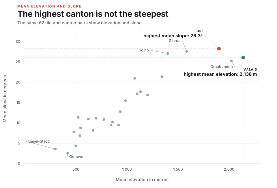
Wrap the DEM column in slope_deg(...), then run the same join and aggregate. The canton ranking changes. Uri has a mean slope of 28.3° and a maximum slope of 72.5°. Valais has a mean slope of 26.1°, but its mean elevation is 237 m higher than Uri's.

Elevation and slope answer different questions, but both use the same 62 pairs:

Use the pattern with other data

The same pattern works with other raster and polygon datasets. For example, replace the DEM with ESA WorldCover. A UDF can mark pixels that contain one type of land cover, such as forest or built-up land. The sum of the marked pixels gives the pixel count for each zone.

The polygons can also represent parcels instead of cantons. The spatial join does not change. Use the geotiff.metadata reader to find the raster tiles that overlap the polygons before opening those tiles.

Raster resolution sets the size of each pixel. A 30 m DEM uses nine times as many pixels as a 90 m DEM to cover the same area. With the 30 m Copernicus DEM, the highest value in Valais is 4,539 m instead of 4,534 m. Both values estimate terrain height from a surface model stored on a grid. The SQL query stays the same.

The main idea

Raster grids and polygon shapes use different data models. Many pipelines join them by exporting data, running a Python script, and saving intermediate files. RS_ZonalStatsAll keeps the join and the statistics in one SQL query. It can read raster data from object storage such as S3.

Use the correct formula for each statistic, and remove pairs with no valid pixels. The same SQL pattern can then process a small set of zones or a large one.

See the RS_ZonalStatsAll reference for all parameters. See the raster tutorial for reading and writing examples. This example contains modified Copernicus DEM data (2026).

Star Apache Sedona on GitHub

A star takes two seconds and helps others discover the projects.

apache/sedona apache/sedona-db apache/sedona-spatialbench