🎉 Apache Sedona 1.9.1 已正式发布!🗺️ 新增 Geography SQL 函数、Box2D 与 Box3D 类型、栅格 Python UDF 等。查看发布说明 →

The official source for Apache Sedona news, technical insights, release updates, and best practices in large-scale spatial data management.

GROUP BY, But for Pixels

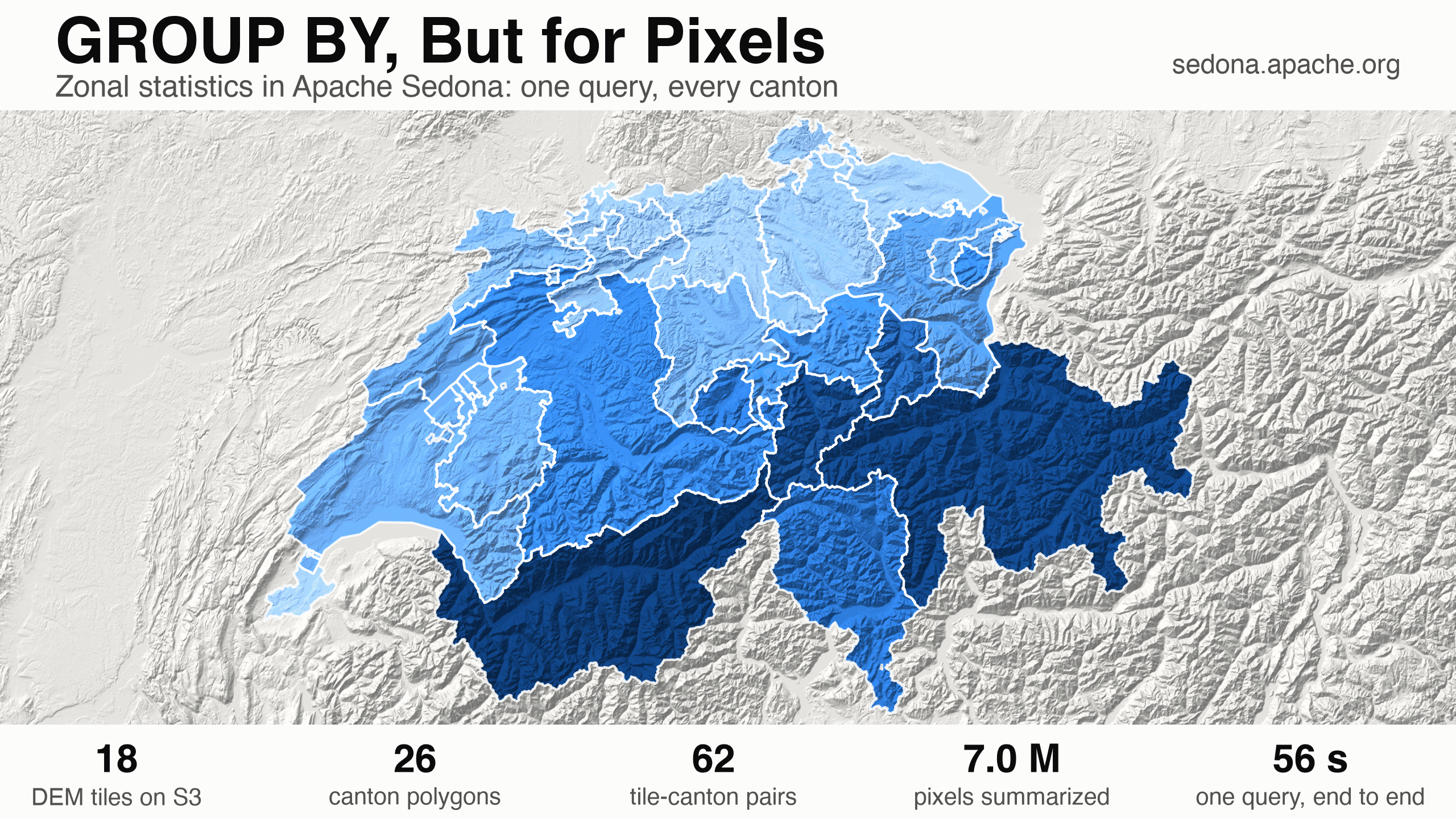
Many raster analyses need one result for each polygon. Examples include mean elevation by canton, forest cover by district, and flood depth by parcel. A raster stores values in a grid of pixels. A polygon defines an area, also called a zone.

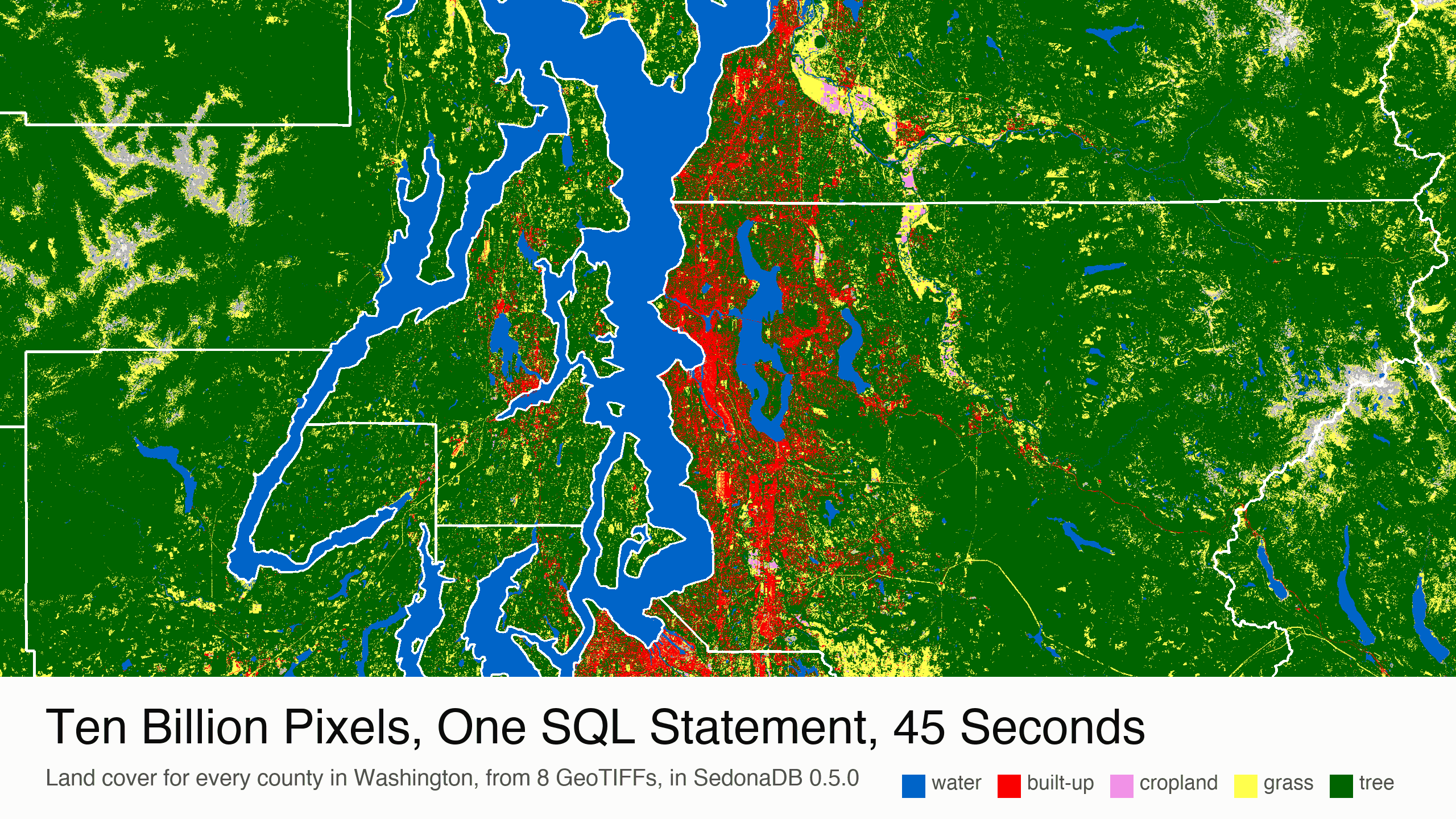
Zonal statistics summarize the raster pixels inside each zone. A spatial join matches data by location. Apache Sedona performs both steps in one query. This example reads 7,006,027 elevation pixels from Amazon S3 and summarizes all 26 Swiss cantons in 56 seconds.

Map of Switzerland. Each canton is shaded by its mean elevation. Low cantons are light blue. Valais and Graubünden are dark blue.

One More Dimension: Apache Sedona Enters the 3D World

In a flat spatial query the world is only its noon shadow on the ground. Two objects whose shadows touch can be four hundred feet apart, and from a flat predicate the answer is the same for both.

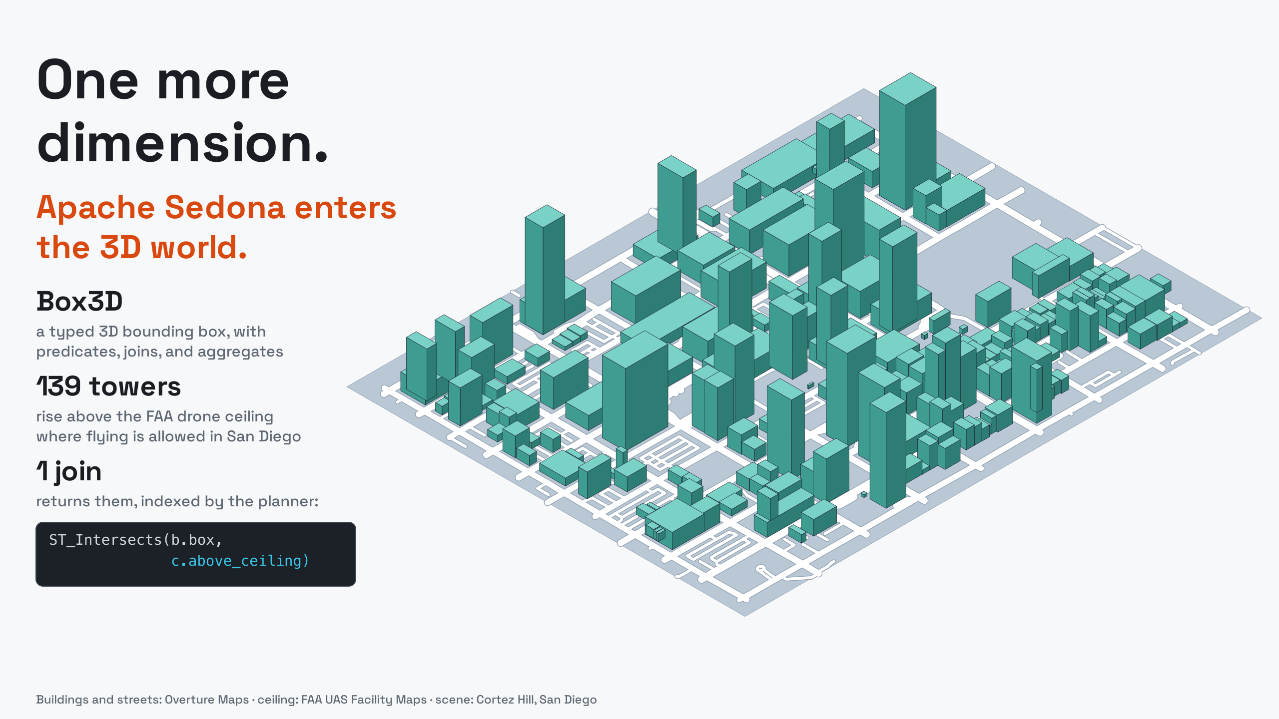
The questions put to spatial engines have stopped being flat. Drones under FAA ceilings, aircraft over towers, apartments above restaurants, mineral deposits below mining leases: each one comes down to whether two volumes meet, and until now the SQL answer was the shadow version. Sedona 1.9.1 adds the missing axis. There is a Box3D type with constructors and accessors, 3D predicates and distances, a 3D extent aggregate, and query plans that account for the third axis.

The cover: an isometric drawing of a San Diego neighborhood, its street grid on the ground and every building rendered as an extruded box, beside the post title

Find the Middle of the Mississippi

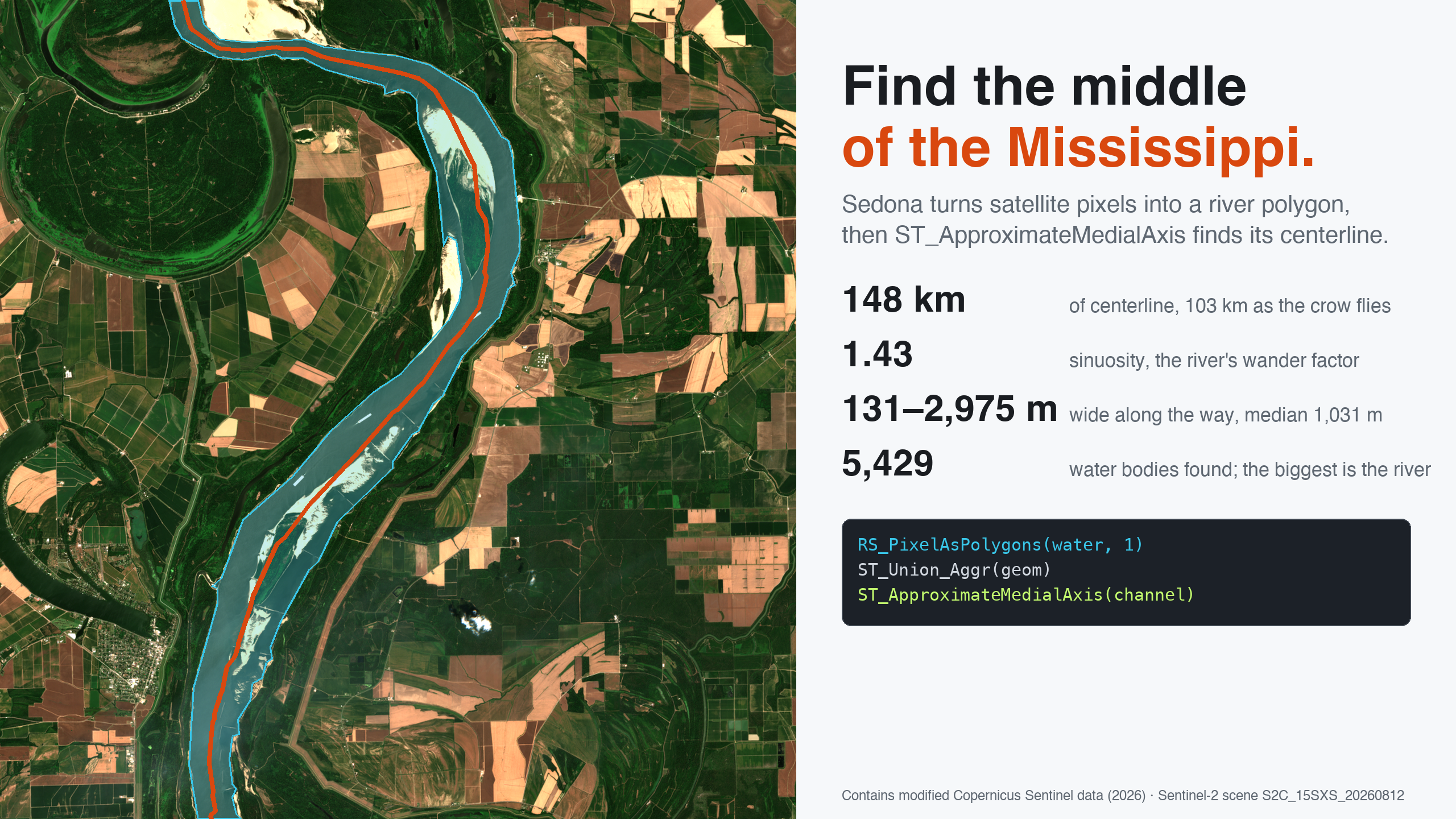
The Mississippi wanders. Between the two edges of a single Sentinel-2 scene it travels 147.6 km to cover 103 km of ground, and its width swings from 131 m to almost 3 km. Every one of those numbers came out of raw pixels: Apache Sedona's raster operators built the river polygon, and ST_ApproximateMedialAxis drew the line down the middle of it.

A Sentinel-2 view of the Mississippi's meanders near Greenville, Mississippi, with the detected river polygon in cyan and its computed centerline in orange; a stats panel lists 148 km of centerline, sinuosity 1.43, widths from 131 to 2,975 m, and the 5,429 water bodies found in the scene

Seven Lines of NumPy, 121 Million Pixels

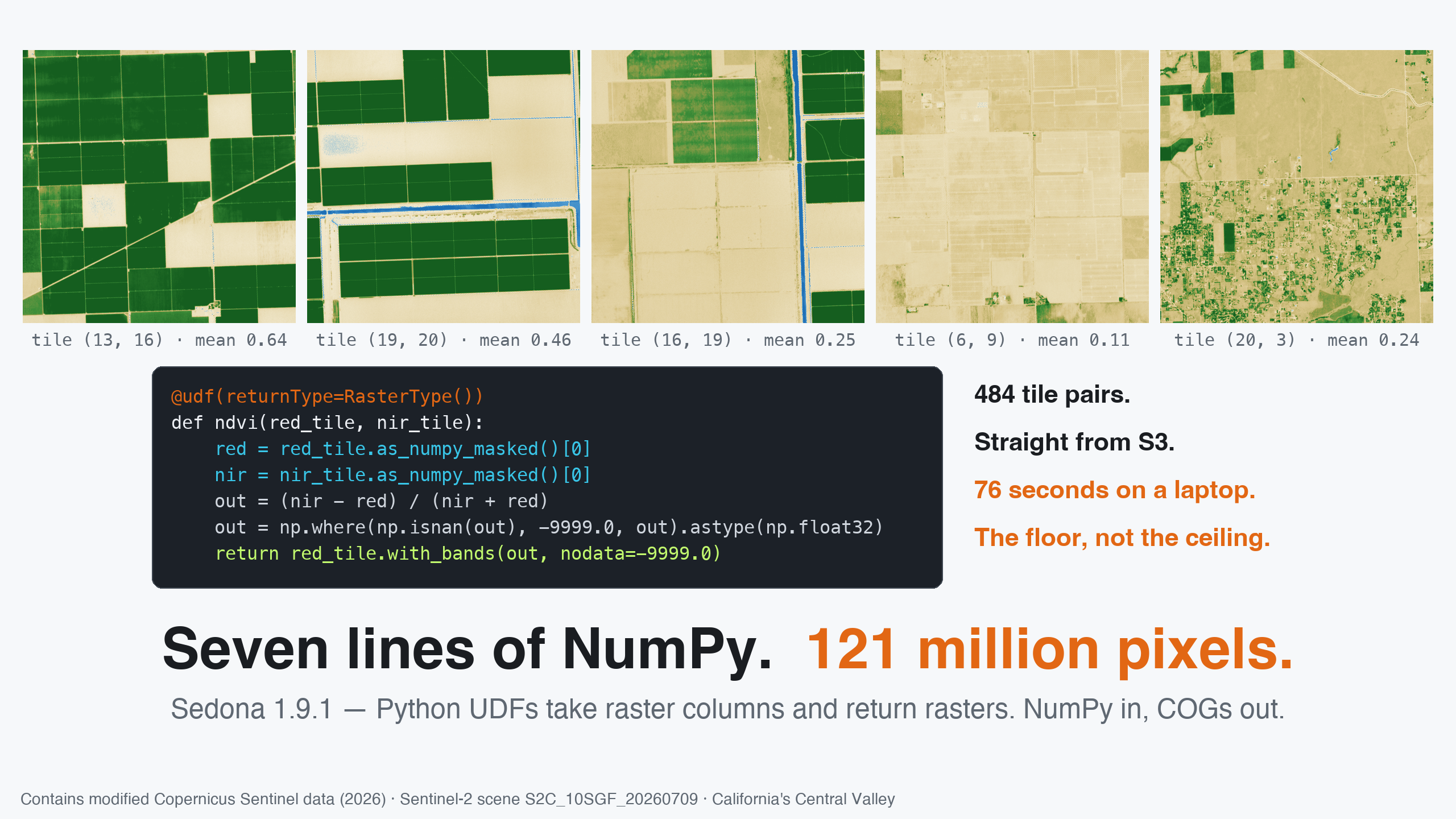
Those deep-green grids are California's Central Valley — some of the most intensively farmed land on Earth, not as a camera sees it but as the NDVI vegetation index does: computed, pixel by pixel, by seven lines of NumPy. Sedona ran those seven lines on 484 satellite tiles in parallel, straight out of a public S3 bucket, and wrote the answer back as Cloud Optimized GeoTIFFs. That's the new move in Sedona 1.9.1: a plain Python UDF can take raster columns and return rasters. If the raster function you need isn't built in — your index, your QA rule, your model — write it.

Five NDVI tiles computed by the seven-line Python UDF — deep-green field grids, blue canals, sandy rangeland, a city — above the UDF's code on a card

Index a Million Rasters Without Reading a Pixel

Every raster team has the bucket. Thousands of GeoTIFFs accumulated from surveys, vendors, and pipelines — and no catalog. Which files cover this area? Which CRS are they in? Which ones were never converted to Cloud Optimized GeoTIFF? Until now, answering meant crawling the bucket with one-off scripts — or pulling rasters down just to inspect them.

Real Sentinel-2 scenes above the metadata card Sedona actually read — index a million rasters, read zero pixels

Your Map Has Hotspots. Prove It.

Anyone can look at a map and see clumps. The interesting questions are the ones eyeballing can't answer: is that clustering statistically real? Exactly where is it significant? And which points genuinely don't belong?

Your map has hotspots — prove it: a field of grid cells with one glowing, statistically significant hotspot, and Sedona's spatial statistics toolkit named beneath

OpenStreetMap, Meet Sedona: Raw .osm.pbf to Spatial SQL

OpenStreetMap is the world's map — every road, café, and coastline, edited by millions of people. It ships as .osm.pbf: a dense, compressed Protocol-Buffers blob of nodes, ways, and relations. Getting that into a cluster usually means a preprocessing detour through osmium or a staging database.

Apache Sedona reads a raw .osm.pbf file straight into a Sedona DataFrame, turning OpenStreetMap nodes, ways, and relations into points and lines