Open Huge GeoTIFFs Without the 2 GB Wall

The hardest part of working with big rasters often isn't the analysis. It's just getting the file open.

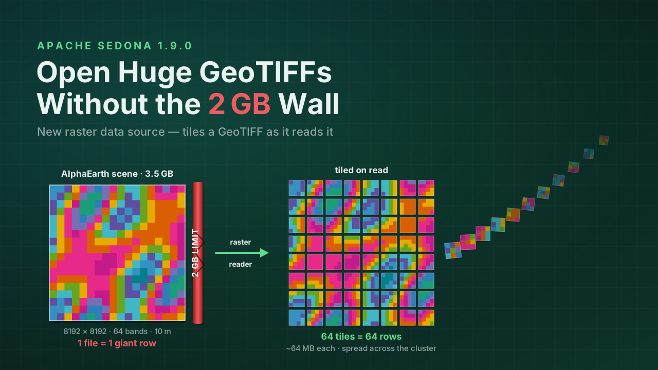
Take a single AlphaEarth Foundations embedding scene — 64 bands of learned satellite features at 10 m resolution, 8192 × 8192 pixels, 3.5 GB in one GeoTIFF. Load it the old way and the job dies — not because your cluster is too small, but because the engine underneath won't materialize a single record larger than 2 GB. Decoded, that raster is over 4 GB; read as one record it becomes a single 4 GB row that topples over before any spatial work begins.

Apache Sedona didn't save you here either: Sedona runs on Spark, so it inherited that ceiling. Its raster loader read each file as one record — one file, one row, one oversized object.

That left the usual ugly workarounds: hand-tile the file first, convert formats offline, or throw memory at the executor and pray.

Tile on read

Apache Sedona 1.9.0 removes the wall. A new raster data source tiles a GeoTIFF as it reads it — one row per tile, streamed straight into a DataFrame:

df = sedona.read.format("raster").load("/data/alphaearth-scene.tiff")

That's the whole thing. The AlphaEarth file is a Cloud Optimized GeoTIFF with 1024 × 1024 internal tiles, so the reader splits it into an 8 × 8 grid — 64 tiles, 64 rows, about 64 MB each — instead of one 4 GB record. Each row carries the tile's raster payload (all 64 embedding bands ride along) plus its (x, y) position in the grid, and Sedona spreads the tiles across the cluster automatically so no single executor has to carry the whole file alone.

+--------------------+---+---+-----------------------+
|                rast|  x|  y| name                  |
+--------------------+---+---+-----------------------+
|GridCoverage2D["g...|  0|  0| alphaearth-scene.tiff |
|GridCoverage2D["g...|  1|  0| alphaearth-scene.tiff |
|GridCoverage2D["g...|  2|  0| alphaearth-scene.tiff |
...

Then it's just a DataFrame

From here it's an ordinary DataFrame — every Sedona raster function runs per tile, across the cluster. First confirm the split, and that each tile still carries all 64 bands at full 1024² resolution:

df.createOrReplaceTempView("aef")

sedona.sql("""
    SELECT COUNT(*)   AS tiles,      -- 64
           MAX(x) + 1 AS tile_cols,  -- 8
           MAX(y) + 1 AS tile_rows   -- 8
    FROM aef
""").show()

sedona.sql("""
    SELECT RS_Width(rast)    AS width,   -- 1024
           RS_Height(rast)   AS height,  -- 1024
           RS_NumBands(rast) AS bands    -- 64
    FROM aef LIMIT 1
""").show()

Then run real analysis. Here's a zonal statistic — the mean of embedding band 1 inside a region of interest — computed the tiling-aware way, because the scene is now 64 rows rather than one:

sedona.sql("""
    WITH zone AS (
        -- ROI polygon, tagged with the scene's CRS (UTM zone 15N) so it
        -- lines up with the raster instead of being read as lon/lat
        SELECT ST_SetSRID(
            ST_GeomFromText(
                'POLYGON((600000 1650000, 640000 1650000, '
                '640000 1700000, 600000 1700000, 600000 1650000))'
            ),
            32615
        ) AS geom
    )
    SELECT SUM(RS_ZonalStats(t.rast, z.geom, 1, 'sum'))
         / SUM(RS_ZonalStats(t.rast, z.geom, 1, 'count')) AS mean_band1
    FROM aef t, zone z
""").show()

On this scene — a 40 km × 50 km ROI at 10 m — that rolls up 20,000,000 pixels spread across the overlapping tiles into one number:

+----------+
|mean_band1|
+----------+
|   82.8633|
+----------+

A single, untiled raster would take RS_ZonalStats(rast, geom, 1, 'mean') directly. With a tiled raster each tile covers only part of the polygon, so you sum the per-tile sum and count and divide once — the same idiom, one extra aggregation. RS_ZonalStatsAll returns every standard statistic in a single call.

A few things worth knowing

• COGs shine here. The AlphaEarth scene above is a Cloud Optimized GeoTIFF; its square 1024 × 1024 internal tiles map cleanly onto the reader, so by default the tile size is taken straight from the file's own tiling scheme — you don't have to specify anything.
• You stay in control. Set option("retile", "false") to load a whole raster as a single row, or set tileWidth / tileHeight to choose the tile size yourself. padWithNoData pads the ragged right and bottom edge tiles out to a uniform size.
• It walks directories too. The reader globs paths and honors the Spark file-source options recursiveFileLookup and pathGlobFilter, so a folder of thousands of scenes is one line.

df = (
    sedona.read.format("raster")
    .option("recursiveFileLookup", "true")
    .option("pathGlobFilter", "*.tif*")
    .load("/data/scenes/")
)

If a file's internal layout isn't tiling-friendly, the reader tells you instead of failing silently — disable tiling with retile=false, set the tile size manually, or translate the file to COG with gdal_translate.

Try it

Whether you work in Earth observation, climate, agriculture, or anything else that ships pixels at scale, this quietly deletes a problem teams have been engineering around for years.

• Walkthrough: Raster data tutorial
• Apache Sedona 1.9.0 release notes