Index a Million Rasters Without Reading a Pixel

Every raster team has the bucket. Thousands of GeoTIFFs accumulated from surveys, vendors, and pipelines — and no catalog. Which files cover this area? Which CRS are they in? Which ones were never converted to Cloud Optimized GeoTIFF? Until now, answering meant crawling the bucket with one-off scripts — or pulling rasters down just to inspect them.

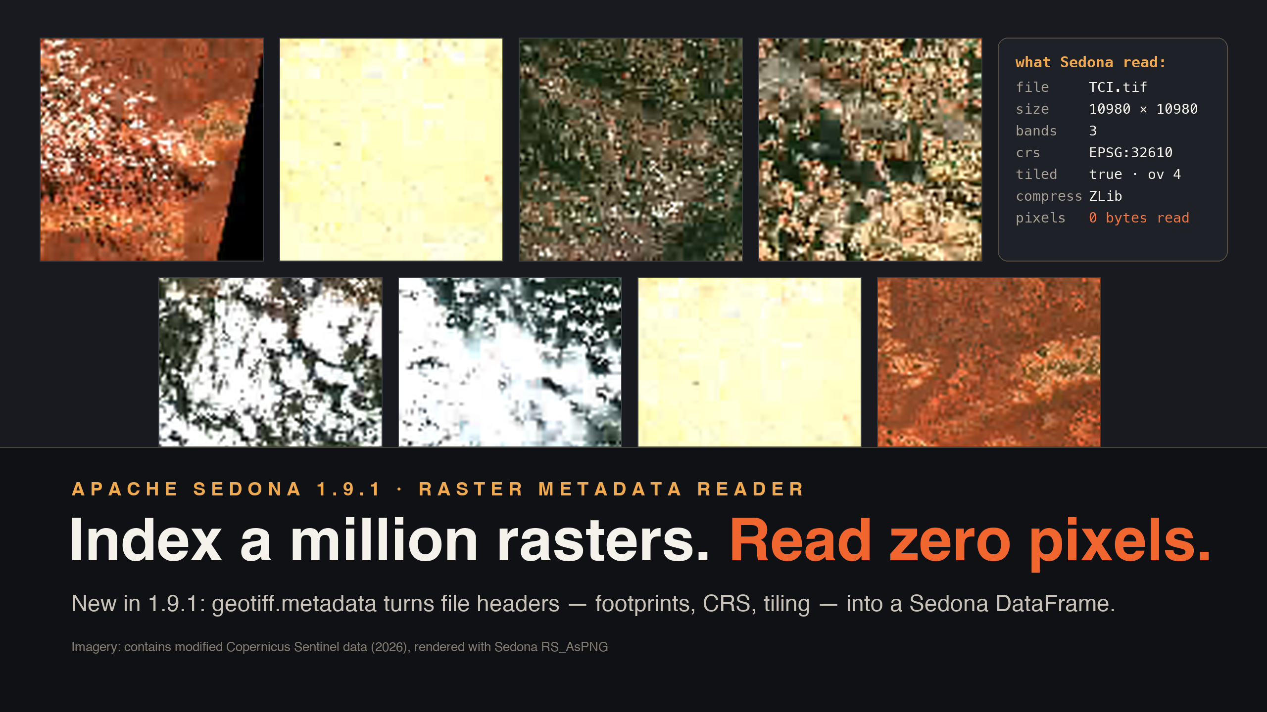
Sedona 1.9.1 ships a pair of raster metadata readers — geotiff.metadata and its sibling netcdf.metadata — that read only the file headers: dimensions, CRS, geotransform, corner coordinates, band layout, tiling, overviews, compression. One row per file, straight into a Sedona DataFrame. The pixels never leave the bucket.

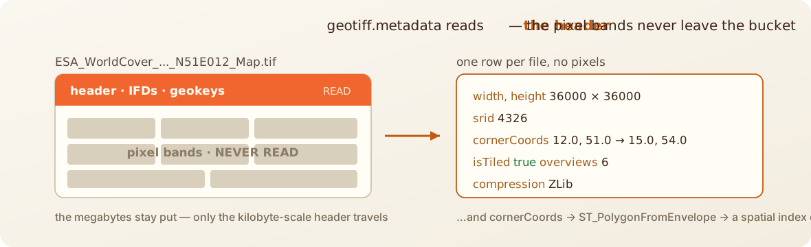
Point it at a bucket

Everything below ran on the released artifacts, exactly as you'd install them — pip install apache-sedona==1.9.1, plus the release jars and S3 support:

from sedona.spark import SedonaContext

config = (
    SedonaContext.builder()
    .master("local[*]")
    .config(
        "spark.jars.packages",
        "org.apache.sedona:sedona-spark-shaded-3.5_2.12:1.9.1,"
        "org.datasyslab:geotools-wrapper:1.9.1-33.5,"
        "org.apache.hadoop:hadoop-aws:3.3.4",
    )
    # the demo bucket is public — read it anonymously
    .config(
        "spark.hadoop.fs.s3a.aws.credentials.provider",
        "org.apache.hadoop.fs.s3a.AnonymousAWSCredentialsProvider",
    )
    .getOrCreate()
)
sedona = SedonaContext.create(config)

For data, we point at a public bucket you have seen before on this blog: s3://sentinel-cogs, the Sentinel-2 COG archive that our STAC post's asset links resolve to. One tile, one month — no catalog service involved, just files:

meta = sedona.read.format("geotiff.metadata").load(
    "s3a://sentinel-cogs/sentinel-s2-l2a-cogs/10/S/EG/2026/6"
)
meta.createOrReplaceTempView("meta")

That's 289 COGs holding 14.7 GB of imagery, indexed in 70 seconds — on a single machine, the worst case for this workload. The scan is an ordinary distributed read: Sedona bin-packs the files across every executor you have, so on a cluster the same line fans out machine-wide and scales with it. What comes back is a table:

sedona.sql("""
    SELECT regexp_extract(path, '([^/]+)$', 1) AS file,
           width, height, numBands, srid, isTiled,
           size(overviews) AS ov, compression,
           ROUND(fileSize / 1048576, 1) AS mb
    FROM meta ORDER BY fileSize DESC LIMIT 3
""").show(truncate=False)

+-------+-----+------+--------+-----+-------+---+-----------+-----+
|file   |width|height|numBands|srid |isTiled|ov |compression|mb   |
+-------+-----+------+--------+-----+-------+---+-----------+-----+
|TCI.tif|10980|10980 |3       |32610|true   |4  |ZLib       |335.9|
|TCI.tif|10980|10980 |3       |32610|true   |4  |ZLib       |330.3|
|TCI.tif|10980|10980 |3       |32610|true   |4  |ZLib       |316.1|
+-------+-----+------+--------+-----+-------+---+-----------+-----+

True-color composites in UTM zone 10N, tiled, four overview levels each — facts we now know without having read a single pixel. The month mixes four raster shapes (10 m, 20 m, 60 m bands and previews), and one GROUP BY sorts them out:

+-----+------+-----+
|width|height|files|
+-----+------+-----+
| 5490|  5490|  119|
|10980|10980 |  102|
| 1830|  1830|   51|
|  343|   343 |  17|
+-----+------+-----+

Built to fan out

The reader is a native Sedona data source, so the usual distributed-scan machinery applies — and it matters more here than usual, because the cost is per-file I/O:

• Many machines, one glob. Files are bin-packed into input partitions and spread across every executor. Ten workers open ten headers at a time; a hundred open a hundred. The 70-second single-machine read above is the floor, not the ceiling.
• Projection pushdown. Header fields are decoded lazily, per column. A query that never touches them — COUNT(*), or a SELECT path inventory — skips header I/O entirely. We measured exactly that on the planetary run below: the pruned count finished in 5.7 seconds while the full header materialization took 12.4 minutes. Select only cornerCoordinates and that's all the reader decodes.
• Limit pushdown. The scan implements Spark's limit pushdown, so .limit(10) while you're exploring stops after ten files instead of sweeping the bucket.
• Partition pruning. If your lake is laid out Hive-style (.../year=2026/sensor=s2/...), those directories surface as columns, and filtering on them skips non-matching files before a single byte is read.

So the honest mental model: listing is nearly free, pruned queries are cheap, and the full header sweep parallelizes to whatever cluster you give it.

The footprint index

The quiet superpower is cornerCoordinates. One expression turns it into a geometry — and suddenly your bucket has a spatial index:

footprints = sedona.sql("""
    SELECT path,
           ST_PolygonFromEnvelope(
               cornerCoordinates.minX, cornerCoordinates.minY,
               cornerCoordinates.maxX, cornerCoordinates.maxY
           ) AS footprint
    FROM meta
""")

WHERE ST_Intersects(footprint, my_aoi) now answers "which files cover this area?" over the whole bucket — the question that used to require a catalog nobody built.

And when you point it at a planet

To see where the ceiling is, we ran the same one-liner over the entire ESA WorldCover archive: every 3°×3° land-cover COG on Earth, in one glob — all 2,651 files, 124 GB of rasters, headers only. Even a single machine an ocean away from the bucket finished in 12.4 minutes; the same scan on a cluster spreads those 2,651 header reads across every worker, so wall-time shrinks with the machines you give it. (You don't need to reproduce this one; the month-sized read above is the same code.)

Plotting nothing but each file's cornerCoordinates draws the continents:

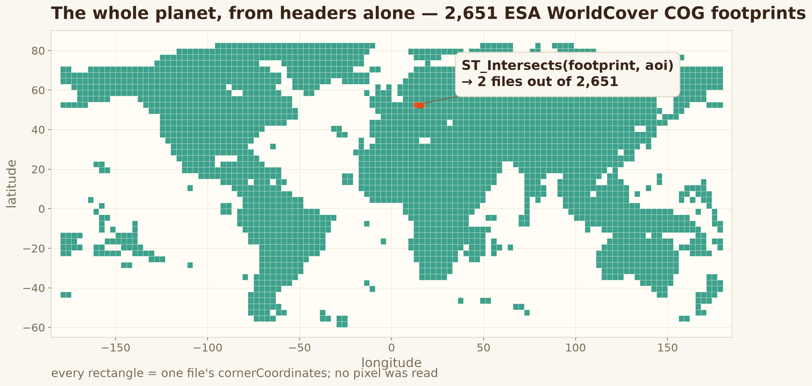
With the index cached, ST_Intersects against an area of interest in western Poland — the Lubusz box from our spatial statistics post — came back in 2.6 seconds with exactly two files:

+--------------------------------------------+
|ESA_WorldCover_10m_2021_v200_N51E015_Map.tif|
|ESA_WorldCover_10m_2021_v200_N51E012_Map.tif|
+--------------------------------------------+

A planetary raster archive, answering spatial questions like a database table.

Audit your raster lake

Metadata is also where data problems hide. To show the audit workflow end to end — reproducibly, offline — we had Sedona generate a deliberately messy 400-file lake with its own raster writers (RS_MakeEmptyRaster → RS_AsGeoTiff / the new RS_AsCOG): 320 plain untiled files, 60 proper COGs, and 20 strays a "web tool" exported in EPSG:3857. Then we indexed it back:

lake = (
    sedona.read.format("geotiff.metadata")
    .option("recursiveFileLookup", "true")
    .load("/data/raster-lake")
)
lake.createOrReplaceTempView("lake")

sedona.sql("""
    SELECT COUNT(*) AS files,
           SUM(CASE WHEN isTiled AND size(overviews) > 0 THEN 1 ELSE 0 END) AS cog_ready,
           SUM(CASE WHEN srid <> 4326 THEN 1 ELSE 0 END) AS crs_strays
    FROM lake
""").show()

+-----+---------+----------+
|files|cog_ready|crs_strays|
+-----+---------+----------+
|  400|       60|        20|
+-----+---------+----------+

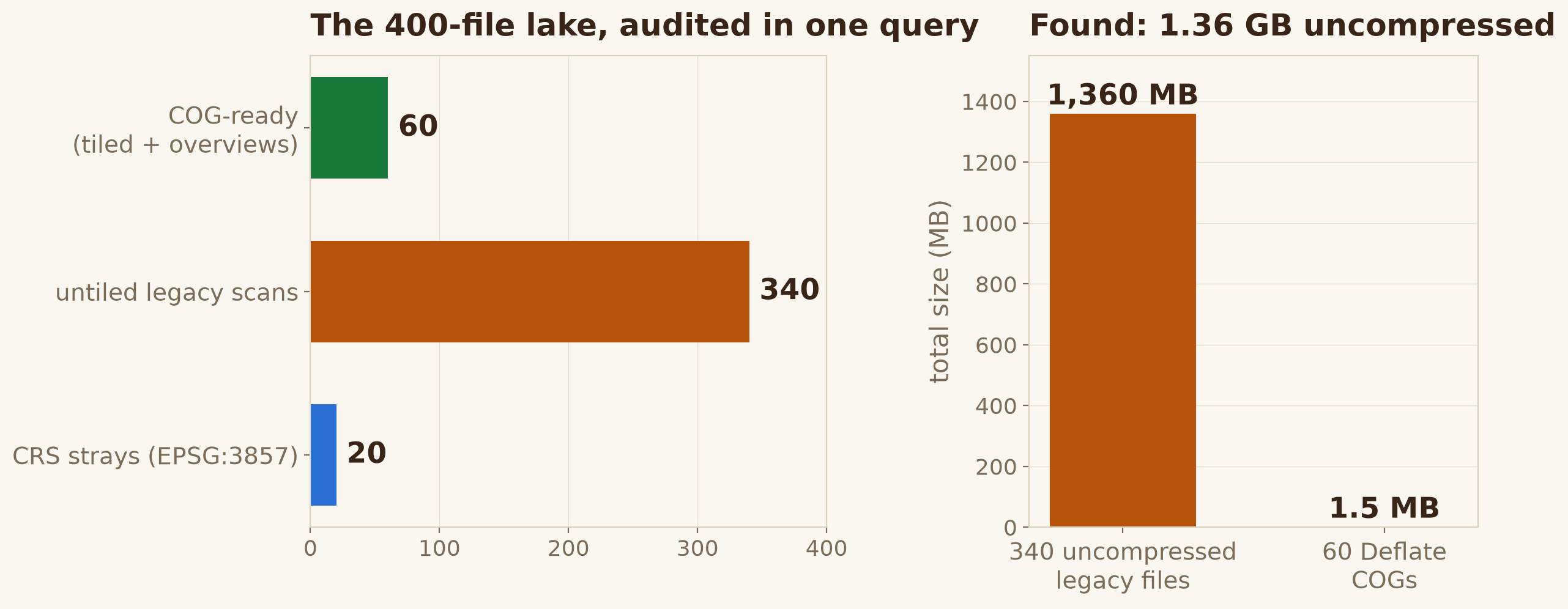
Three lines of SQL and the lake confesses: only 60 files are COG-ready, 20 are quietly in the wrong CRS, and the untiled legacy scans are hoarding 1,360 MB uncompressed (our synthetic tiles are empty, so their compression ratio is theatrical — but the finding is exactly what you'd get on real data: the audit tells you where the storage and correctness debt lives).

NetCDF gets the same treatment

The sibling netcdf.metadata reader does the same for scientific data cubes — variables, dimensions, attributes, and CF grid_mapping translated to a proper CRS — so climate archives can be inventoried the same way. Same pattern: sedona.read.format("netcdf.metadata").load(...).

The point

Catalogs like STAC are wonderful — when someone has built one for you. For every other bucket of rasters, Sedona 1.9.1 turns the files themselves into the catalog: one read for the metadata, one expression for the footprints, plain SQL for the audit. Index a million rasters — and never read a pixel.

Full option reference in the GeoTIFF metadata tutorial and NetCDF metadata tutorial.

Star Apache Sedona on GitHub

A star takes two seconds and helps others discover the projects.

apache/sedona apache/sedona-db apache/sedona-spatialbench