OpenStreetMap, Meet Sedona: Raw .osm.pbf to Spatial SQL
OpenStreetMap is the world's map — every road, café, and coastline, edited by millions of people. It ships as .osm.pbf: a dense, compressed Protocol-Buffers blob of nodes, ways, and relations. Getting that into a cluster usually means a preprocessing detour through osmium or a staging database.
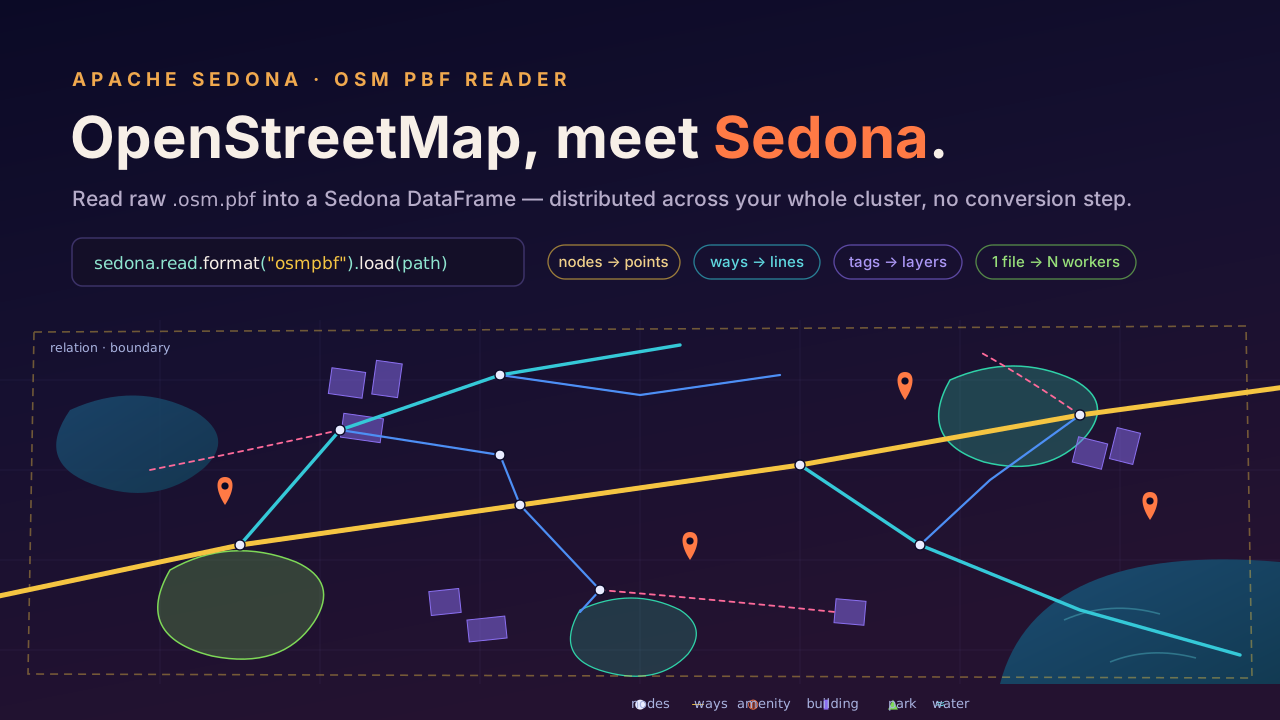
SedonaSpark reads .osm.pbf natively. Point the osmpbf format at a file and you get a Sedona DataFrame of raw OSM elements — no conversion step. And because Sedona is a distributed engine, that one-line read fans out across a cluster: a planet-scale file is just more partitions. From there it's ordinary Spatial SQL: assemble geometries, filter by tag, measure, join. Every snippet below runs against the small Monaco extract that ships in Sedona's test resources, so you can reproduce it verbatim — and scale it up unchanged.
One line to raw OSM
from sedona.spark import SedonaContext

sedona = SedonaContext.create(SedonaContext.builder().master("local[*]").getOrCreate())

# a regional extract from Geofabrik, or Sedona's bundled Monaco sample
osm = sedona.read.format("osmpbf").load(
    "spark/common/src/test/resources/osmpbf/monaco-latest.osm.pbf"
)
osm.createOrReplaceTempView("osm")
osm.printSchema()
The reader gives you the raw OSM element model, one row per element:
 |-- id: long
 |-- kind: string                 (node | way | relation)
 |-- location: struct<longitude, latitude>   -- nodes only
 |-- tags: map<string, string>
 |-- refs: array<long>            -- ordered member node/way ids (ways & relations)
 |-- ref_roles: array<string>
 |-- ref_types: array<string>
 |-- changeset / timestamp / uid / user / version / visible   -- edit metadata
Monaco is small but complete — three element kinds, one table:
sedona.sql("SELECT kind, COUNT(*) AS n FROM osm GROUP BY kind ORDER BY n DESC").show()
+--------+-----+
|kind    |n    |
+--------+-----+
|node    |39587|
|way     | 5777|
|relation|  309|
+--------+-----+
Nodes are points
A node is the only element with a coordinate, so points are immediate. Here are Monaco's amenities:
sedona.sql("""
    SELECT id, tags['amenity'] AS amenity, tags['name'] AS name,
           ST_ReducePrecision(ST_Point(location.longitude, location.latitude), 5) AS geom
    FROM   osm
    WHERE  kind = 'node' AND tags['amenity'] IS NOT NULL
    ORDER BY id LIMIT 5
""").show(truncate=False)
+--------+-------+------------------------------+------------------------+
|id      |amenity|name                          |geom                    |
+--------+-------+------------------------------+------------------------+
|25191432|parking|Parking du Chemin des Pêcheurs|POINT (7.42711 43.73128)|
|25230434|fuel   |Esso                          |POINT (7.41209 43.72851)|
|25239190|parking|null                          |POINT (7.42919 43.74531)|
|25239191|parking|Parking du centre commercial  |POINT (7.41792 43.7309) |
|25249199|parking|Parking de la Gare            |POINT (7.41908 43.7389) |
+--------+-------+------------------------------+------------------------+
Ways are just node IDs — assemble the lines
Here's the part that trips people up. A way (a road, a river, a building outline) has no coordinates of its own — only refs, an ordered list of the node IDs it passes through. To get a geometry you resolve those IDs back to node coordinates, in order, and connect them.
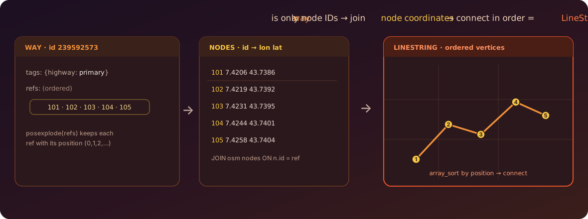
That's a posexplode to keep the ordering, a join to the nodes, and a rebuild in sequence:
roads = sedona.sql("""
    WITH nodes AS (
        SELECT id, location.longitude AS lon, location.latitude AS lat
        FROM osm WHERE kind = 'node'
    ),
    way_pts AS (                               -- one row per (way, vertex), ordered
        SELECT w.id AS way_id, w.highway, w.pos AS seq, n.lon, n.lat
        FROM (SELECT id, tags['highway'] AS highway, posexplode(refs) AS (pos, ref)
              FROM osm WHERE kind = 'way' AND tags['highway'] IS NOT NULL) w
        JOIN nodes n ON n.id = w.ref
    )
    SELECT way_id, highway,
           ST_MakeLine(
               transform(array_sort(collect_list(struct(seq, lon, lat))),
                         x -> ST_Point(x.lon, x.lat))
           ) AS geom
    FROM   way_pts
    GROUP BY way_id, highway
    HAVING count(*) >= 2
""")
roads.createOrReplaceTempView("roads")
array_sort on (seq, …) guarantees the vertices land in the way's declared order, and ST_MakeLine connects the sorted points into the geometry — no string assembly. Note the tag filter sits before the join, so only road vertices are ever shuffled. Now the ways are real LineStrings and the full Spatial SQL toolkit applies. How much road is in Monaco?
sedona.sql("""
    SELECT highway,
           COUNT(*) AS ways,
           ROUND(SUM(ST_LengthSpheroid(geom)) / 1000, 1) AS km
    FROM   roads
    GROUP BY highway
    ORDER BY km DESC
    LIMIT 5
""").show(truncate=False)
+-----------+----+----+
|highway    |ways|km  |
+-----------+----+----+
|footway    |1612|63.5|
|residential| 311|29.0|
|service    | 379|19.6|
|tertiary   | 127|10.6|
|secondary  | 174|10.5|
+-----------+----+----+
3,334 road ways, 163.9 km of it — reconstructed from raw node references, no preprocessing. (The same pattern builds rivers, boundaries, or coastlines; you just filter a different tag.)
Every element carries its history
OSM elements are versioned. Each row keeps a version and an edit timestamp, so you can measure how alive a map is — no separate history file. When was Monaco mapped?
sedona.sql("""
    SELECT YEAR(timestamp) AS yr, COUNT(*) AS edits
    FROM   osm WHERE timestamp IS NOT NULL
    GROUP BY YEAR(timestamp) ORDER BY edits DESC LIMIT 5
""").show()
+----+-----+
|  yr|edits|
+----+-----+
|2023| 8595|
|2011| 5206|
|2022| 5175|
|2024| 4110|
|2020| 3865|
+----+-----+
And which features have been revised the most? version tells you — the big administrative-boundary relations churn constantly:
sedona.sql("""
    SELECT kind, tags['name'] AS name, version
    FROM   osm WHERE tags['name'] IS NOT NULL
    ORDER BY version DESC LIMIT 3
""").show(truncate=False)
+--------+--------------------------+-------+
|kind    |name                      |version|
+--------+--------------------------+-------+
|relation|France métropolitaine     |800    |
|relation|Provence-Alpes-Côte d'Azur|774    |
|relation|France (terres)           |614    |
+--------+--------------------------+-------+
A note on the metadata fields
The reader also exposes user, uid, and changeset. Public Geofabrik extracts strip these for privacy, so they arrive empty — as they do here. To analyze contributors by name you need a full-history or internal planet file; timestamp and version are always present.
Built for the planet, not the demo
Monaco is a teaching extract — the full OpenStreetMap planet is a single .osm.pbf of roughly 80 GB holding billions of elements. Three properties of the reader make that size a non-event on a Sedona cluster:
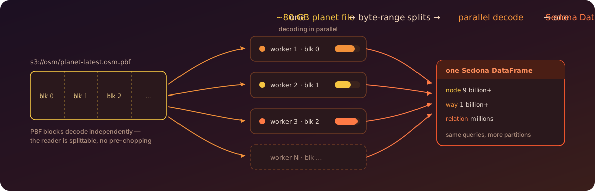
- One file, many workers. PBF is a sequence of independently decodable blocks, and the reader declares the format splittable — Sedona carves even a single planet file into byte-range partitions and decodes them in parallel across the cluster. No pre-chopping into per-region files.
- Object storage native. The same
load()reads from S3 or HDFS as happily as from a local disk, so the planet file never has to leave your bucket. - Assembly is a join, not a script. The refs → coordinates rebuild above is an ordinary distributed join between two slices of the same table. Where a single-machine tool streams the planet through one process, Sedona shuffles the work across however many machines you give it — the classic way OSM processing becomes horizontal instead of overnight.
The result: the four queries in this post run against planet-latest.osm.pbf exactly as written — just with more partitions underneath.
The point
.osm.pbf stops being a format problem. One osmpbf read turns the planet's map into a Sedona DataFrame; posexplode + a join reconstitutes geometries from raw references; and from there OpenStreetMap is just another spatial table — one you can filter, measure, and join at whatever scale your cluster allows.
Grab any regional extract from Geofabrik — or the planet itself — and point the reader at it: the queries above scale from Monaco to the whole world unchanged.
Star Apache Sedona on GitHub
A star takes two seconds and helps others discover the projects.