Find the Middle of the Mississippi
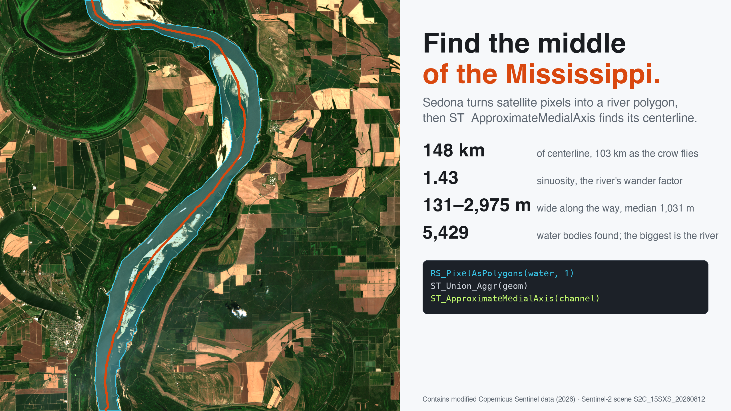
The Mississippi wanders. Between the two edges of a single Sentinel-2 scene it travels 147.6 km to cover 103 km of ground, and its width swings from 131 m to almost 3 km. Every one of those numbers came out of raw pixels: Apache Sedona's raster operators built the river polygon, and ST_ApproximateMedialAxis drew the line down the middle of it.
From pixels to a polygon
The scene is a cloud-free August capture of the river near Greenville, MS, from the Sentinel-2 COG archive that last week's NDVI post used. The start is the same: two bands of about 200 MB each, read as 512-pixel tiles and paired on tile position.
scene = (
    "s3a://sentinel-cogs/sentinel-s2-l2a-cogs/15/S/XS/2026/8/"
    "S2C_15SXS_20260812_0_L2A"
)
reader = (
    sedona.read.format("raster").option("tileWidth", "512").option("tileHeight", "512")
)
green_df = reader.load(f"{scene}/B03.tif")
nir_df = reader.load(f"{scene}/B08.tif")

tiles = green_df.select(col("rast").alias("green"), "x", "y").join(
    nir_df.select(col("rast").alias("nir"), "x", "y"), ["x", "y"]
)
Session setup: released artifacts, anonymous S3
import numpy as np
from pyspark.sql.functions import col, udf

from sedona.spark import SedonaContext
from sedona.spark.sql.types import RasterType

config = (
    SedonaContext.builder()
    .master("local[4]")
    .config("spark.driver.memory", "8g")
    .config(
        "spark.jars.packages",
        "org.apache.sedona:sedona-spark-shaded-3.5_2.12:1.9.1,"
        "org.datasyslab:geotools-wrapper:1.9.1-33.5,"
        "org.apache.hadoop:hadoop-aws:3.3.4",
    )
    .config(
        "spark.hadoop.fs.s3a.aws.credentials.provider",
        "org.apache.hadoop.fs.s3a.AnonymousAWSCredentialsProvider",
    )
    .config("spark.hadoop.fs.s3a.bucket.sentinel-cogs.endpoint.region", "us-west-2")
    .getOrCreate()
)
sedona = SedonaContext.create(config)
Water reflects more green light than near-infrared. That makes the water index a seven-line Python UDF, the same shape as last week's NDVI function:
@udf(returnType=RasterType())
def ndwi(green_tile, nir_tile):
    g = green_tile.as_numpy_masked()[0]
    n = nir_tile.as_numpy_masked()[0]
    out = (g - n) / (g + n)
    out = np.where(np.isnan(out), -9999.0, out).astype(np.float32)
    return green_tile.with_bands(out, nodata=-9999.0)


tiles.withColumn("ndwi", ndwi(col("green"), col("nir"))).createOrReplaceTempView(
    "ndwi_tiles"
)
Now the raster ops. A kilometre-wide river does not need 10 m pixels, so RS_Resample drops each tile to 40 m and cuts the polygon count downstream by sixteen. RS_PixelAsPolygons turns every wet pixel into a square, and one ST_Union_Aggr per tile dissolves the squares. The per-tile union keeps the job distributed: 484 small unions spread across the cluster instead of one giant one.
WITH small AS (
    SELECT x, y, RS_Resample(ndwi, 128, 128, false, 'Bilinear') AS r FROM ndwi_tiles
),
px AS (
    SELECT x, y, explode(RS_PixelAsPolygons(r, 1)) AS p FROM small
)
SELECT x, y, ST_Union_Aggr(p.geom) AS geom
FROM px WHERE p.value > 0.0
GROUP BY x, y
That step produces 410 tile-polygons. One more union and an ST_Dump give every water body its own row:
WITH all_water AS (SELECT ST_Union_Aggr(geom) AS geom FROM tile_water),
bodies AS (SELECT explode(ST_Dump(geom)) AS geom FROM all_water)
SELECT ROUND(ST_Area(geom) / 1e6, 1) AS km2, ST_NPoints(geom) AS vertices,
       ST_NumInteriorRings(geom) AS islands
FROM bodies ORDER BY km2 DESC LIMIT 5
+-----+--------+-------+
|  km2|vertices|islands|
+-----+--------+-------+
|157.4|   17530|    179|
| 16.5|    1572|     21|
| 14.9|    1365|      6|
| 10.7|     990|      5|
|  7.9|     776|      1|
+-----+--------+-------+
The scene holds 5,429 water bodies: oxbow lakes, catfish ponds, borrow pits. The biggest one, by a mile, is the river: 157 km² of water with 179 islands and sandbars punched through it.
Find the middle
ST_ApproximateMedialAxis computes a polygon's straight skeleton and keeps the interior edges, which is the centerline. Two preprocessing steps reduce work and noise: simplify the stair-stepped boundary, since skeleton cost climbs steeply with vertex count, then remove holes so islands do not create loops in the skeleton. The query below smooths the outline with a buffer out and back in, simplifies it to 80 m, keeps the exterior ring, then skeletonizes and merges the pieces.
WITH river AS (SELECT geom FROM bodies ORDER BY ST_Area(geom) DESC LIMIT 1),
clean AS (
    SELECT ST_MakePolygon(ST_ExteriorRing(
               ST_SimplifyPreserveTopology(ST_Buffer(ST_Buffer(geom, 60), -60), 80)
           )) AS channel
    FROM river
)
SELECT channel, ST_LineMerge(ST_ApproximateMedialAxis(channel)) AS axis FROM clean
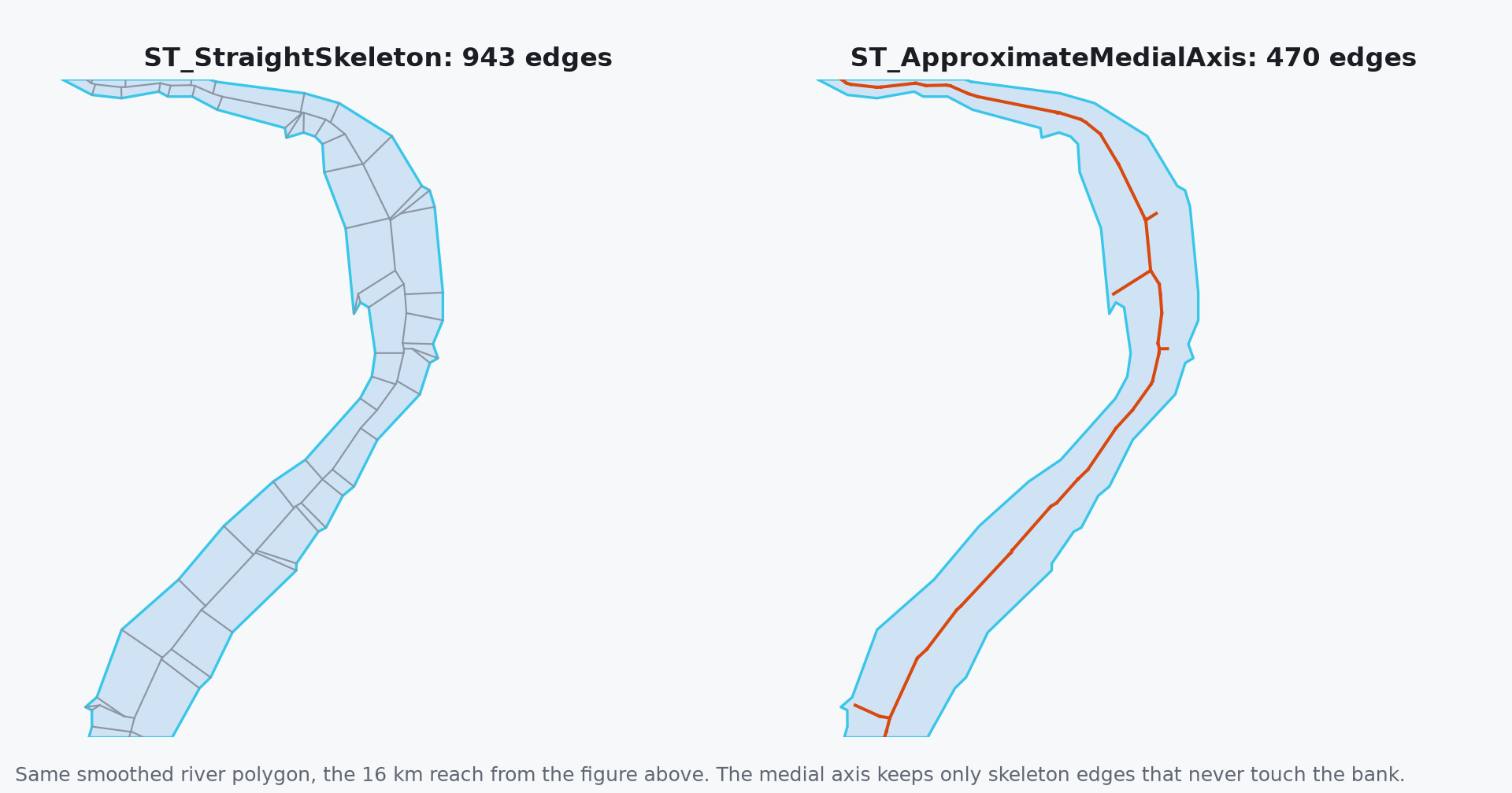
17,530 vertices become 474, and the medial axis returns 470 raw edges, 81 line parts after ST_LineMerge, 205 km of skeleton including every spur into a side channel or around a sandbar.
Under the hood, ST_ApproximateMedialAxis is built on ST_StraightSkeleton, which shrinks every edge of the polygon inward at the same speed and records where the edges meet. On this channel the straight skeleton has 943 edges and 437.7 km of line: ribs run from every bend in the bank to the spine. The medial axis keeps the 470 edges that never touch the bank. Call ST_StraightSkeleton directly when the ribs are the point, as in roof modeling or polygon offsetting.
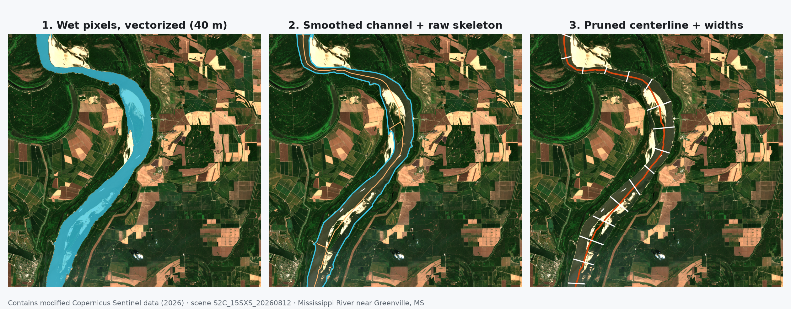
The spurs come off with a pruning rule in SQL: a line part survives if it is at least 10 km long or if both of its ends touch another part. Three rounds of that rule, each followed by ST_LineMerge, leave a single line.
WITH parts AS (SELECT posexplode(ST_Dump(axis)) AS (id, g) FROM centerline),
tips AS (
    SELECT id, g, ST_StartPoint(g) AS s, ST_EndPoint(g) AS e, ST_Length(g) AS len FROM parts
),
kept AS (
    SELECT a.g FROM tips a
    WHERE a.len >= 10000
       OR (EXISTS (SELECT 1 FROM tips b WHERE b.id <> a.id AND ST_Intersects(b.g, a.s))
           AND EXISTS (SELECT 1 FROM tips b WHERE b.id <> a.id AND ST_Intersects(b.g, a.e)))
)
SELECT ST_LineMerge(ST_Union_Aggr(g)) AS axis FROM kept
SELECT ST_NumGeometries(main) AS parts,
       ROUND(ST_Length(main) / 1000, 1) AS km,
       ROUND(ST_Distance(ST_StartPoint(main), ST_EndPoint(main)) / 1000, 1) AS straight_km,
       ROUND(ST_Length(main) / ST_Distance(ST_StartPoint(main), ST_EndPoint(main)), 2) AS sinuosity
FROM main
+-----+-----+-----------+---------+
|parts|   km|straight_km|sinuosity|
+-----+-----+-----------+---------+
|    1|147.6|      103.4|     1.43|
+-----+-----+-----------+---------+
The Mississippi runs 147.6 km through this 110 km scene. Its two ends sit 103.4 km apart. Sinuosity 1.43: the river travels 43 percent farther than a straight line would.
How wide is it?
With a centerline and a bank, width is a distance query. Step along the centerline every 2 km, and at each point take twice the distance to the nearest bank:
WITH steps AS (
    SELECT explode(sequence(1000, CAST(ST_Length(main) AS INT), 2000)) AS d, main, channel
    FROM centerline
),
pts AS (
    SELECT d, ST_LineInterpolatePoint(main, d / ST_Length(main)) AS pt, channel FROM steps
)
SELECT COUNT(*) AS samples, MIN(w) AS narrowest_m, percentile(w, 0.5) AS median_m, MAX(w) AS widest_m
FROM (SELECT ROUND(2 * ST_Distance(pt, ST_Boundary(channel)), 0) AS w FROM pts)
+-------+-----------+--------+--------+
|samples|narrowest_m|median_m|widest_m|
+-------+-----------+--------+--------+
|     74|      131.0|  1031.5|  2975.0|
+-------+-----------+--------+--------+
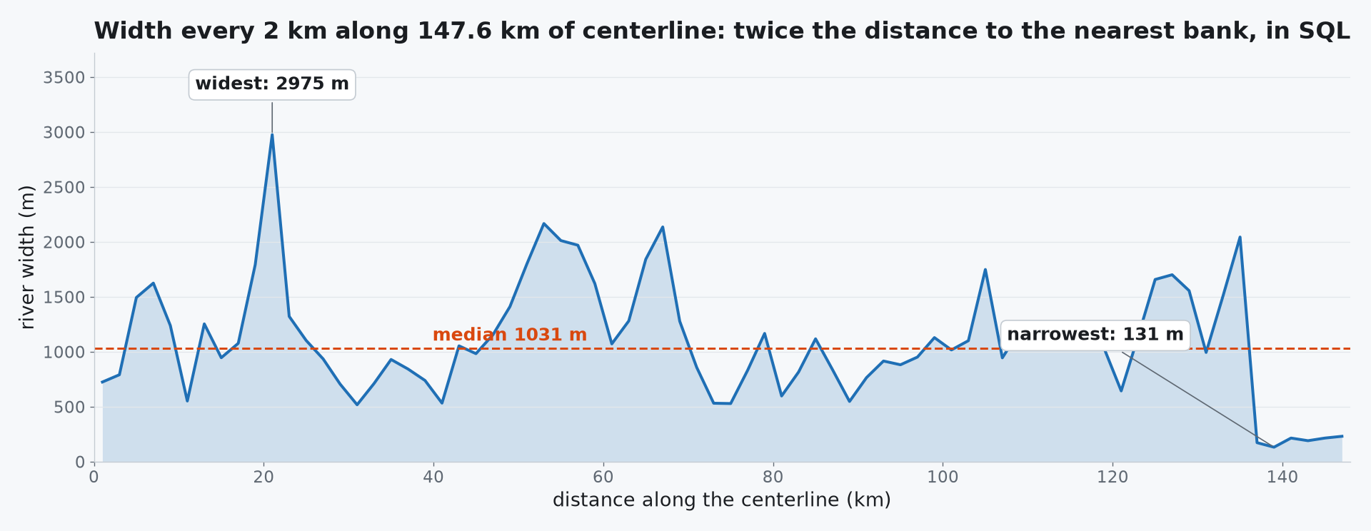
The river is about a kilometre wide for most of the reach and close to three kilometres where the channel balloons around mid-river bars. The final 12 km drop to about 200 m: there the 10 km rule kept a long side channel at the scene edge over the main channel's shorter last reach, and the 131 m minimum sits in that side channel. Every number comes from the pixels of one scene, read straight from S3.
How the pipeline distributes work
Every stage of this pipeline is a table of rows, and Sedona spreads rows across executors. After the band join, the UDF, the resampling, and the per-tile unions run independently on each executor. Skeletonization runs once per water-body row; this scene produced 5,429 such rows, and the SQL does not change when a larger input produces more. The global union is the remaining aggregation point, and larger workloads can partition that union by region.
One detail shapes the plan: the raster reader emits a file's tiles from a single task, so the fan-out begins at the join. The centerline comes out as an ordinary geometry column. Index it with the geotiff.metadata footprints, join it to gauges and bridges, write it to GeoParquet.
Roads are next
The same pipeline, mask to polygons to union to medial axis, can apply to other sufficiently wide polygonal features, including roads. Road networks are the next target, and they come with their own lessons: a road needs several pixels of width before a skeleton can find it, and a street grid is made of holes that the pipeline has to keep. Roads get their own post next week.
Function references: ST_ApproximateMedialAxis, RS_PixelAsPolygons, RS_Resample. The UDF pattern is in the Raster UDF reference.
Star Apache Sedona on GitHub
A star takes two seconds and helps others discover the projects.