Working with Zarr and NDArray data in SedonaDB
SedonaDB's raster type is N-dimensional: a band isn't limited to a 2-D (y, x) grid — it can carry additional axes such as time, year, or band. This makes it a natural fit for datacubes: climate reanalyses, satellite time series, and model outputs.
The sedonadb-zarr extension reads Zarr groups (v2 or v3) — local or in cloud object storage — directly into that raster type, so a datacube becomes a table you can query.
This page walks through loading a real Zarr datacube from object storage, inspecting its dimensions, slicing out a 2-D plane, drawing its chunk grid on a map, and handing a plane to NumPy.
Install
sedonadb-zarr is an extension, distributed separately from the core SedonaDB package. The examples below also use sedonadb-expr (which adds the .rst raster accessor used in the DataFrame expressions) and, for the map, lonboard:
pip install "apache-sedona[db]" sedonadb-zarr sedonadb-expr lonboard
lonboard is only needed for the map at the end; everything else works without it.
Connect and load
Register the extension on your connection, then read a Zarr group. We'll use a public, anonymously readable cube: ERA5 rainfall over 2015–2020, stored as a multiscale Zarr pyramid in EPSG:3857. We read one pyramid level and the rain_ok rainfall array:
import sedona.db
import sedonadb_zarr

sd = sedona.db.connect()
sd.register(sedonadb_zarr.ZarrExtension())

url = "https://weathermapdata.rdrn.me/era5_2015_2020_l5.zarr/2"
# The path doesn't end in `.zarr`, so name the format. `arrays` selects the
# data array to read (the group also holds coordinate / CRS variables).
spec = sedonadb_zarr.Zarr().with_options({"arrays": ["rain_ok"]})
cube = sd.read(url, format=spec)
When a group's path does end in .zarr and needs no options, you can name the format with the string shorthand instead: sd.read(uri, format="zarr").
sedonadb-zarr emits one row per Zarr chunk, so the storage layout is the data layout. This level tiles its 512 × 512 grid into a 4 × 4 grid of 128 × 128 chunks, and the cube is chunked one year per chunk — so it loads as 16 × 6 = 96 rows, each a single year of one spatial tile:
cube.count()
96
Inspect the dimensions
The dimension accessors read the raster's schema only — no pixel data is loaded — so they return near-instantly even against a large remote cube. Each row reports its chunk's shape, not the full cube extent. All chunks share the same shape here, so we look at one:
cube.select(
    cube.raster.rst.num_dimensions().alias("ndim"),
    cube.raster.rst.dim_names().alias("dims"),
    cube.raster.rst.shape().alias("shape"),
    cube.raster.rst.dim_size("year").alias("n_year"),
).show(1)
┌───────┬──────────────┬───────────────┬────────┐
│  ndim ┆     dims     ┆     shape     ┆ n_year │
│ int32 ┆     list     ┆      list     ┆  int64 │
╞═══════╪══════════════╪═══════════════╪════════╡
│     3 ┆ [year, y, x] ┆ [1, 128, 128] ┆      1 │
└───────┴──────────────┴───────────────┴────────┘
Each chunk is 3-dimensional ([year, y, x]) with a 128 × 128 spatial footprint — one tile of the full 512 × 512 grid. n_year = 1 because the cube is chunked one year per chunk: a single row carries one year of one tile.
Slice out a 2-D plane
RS_Slice selects a single index along a named dimension and drops it. Here each chunk's year axis has length 1, so slicing index 0 collapses it, turning every [1, 128, 128] chunk into a 2-D [y, x] plane — the tile's rainfall field for its year:
sliced = cube.select(plane=cube.raster.rst.slice("year", 0))
sliced.select(
    dims=sliced.plane.rst.dim_names(),
    shape=sliced.plane.rst.shape(),
).show(1)
┌────────┬────────────┐
│  dims  ┆    shape   │
│  list  ┆    list    │
╞════════╪════════════╡
│ [y, x] ┆ [128, 128] │
└────────┴────────────┘
RS_Slice needs pixel data, so SedonaDB resolves each row's Zarr chunk on demand before slicing — you never call a loader yourself.
Related accessors reshape a cube in other ways:
cube.raster.rst.slice_range(dim, start, end)keeps a contiguous range of a dimension instead of a single index.cube.raster.rst.dim_to_band(dim)/cube.raster.rst.band_to_dim(name)move an axis between the dimension list and the band list.
See where the chunks are — on a map
Every row is a chunk with a real, georeferenced footprint (the cube declares EPSG:3857), so RS_Envelope turns a chunk into its bounding geometry without decoding a single pixel. Reproject the footprints to lon/lat and you can draw the chunk grid straight onto a map:
from lonboard import viz  # in a notebook with lonboard installed

f = sd.funcs
chunks = cube.select(geom=f.st_transform(cube.raster.rst.envelope(), "EPSG:4326"))

# Draw outlines only, so the basemap shows through the chunk grid.
viz(
    chunks,
    polygon_kwargs=dict(
        filled=False,
        stroked=True,
        get_line_color=[236, 64, 160],
        line_width_min_pixels=2,
    ),
)
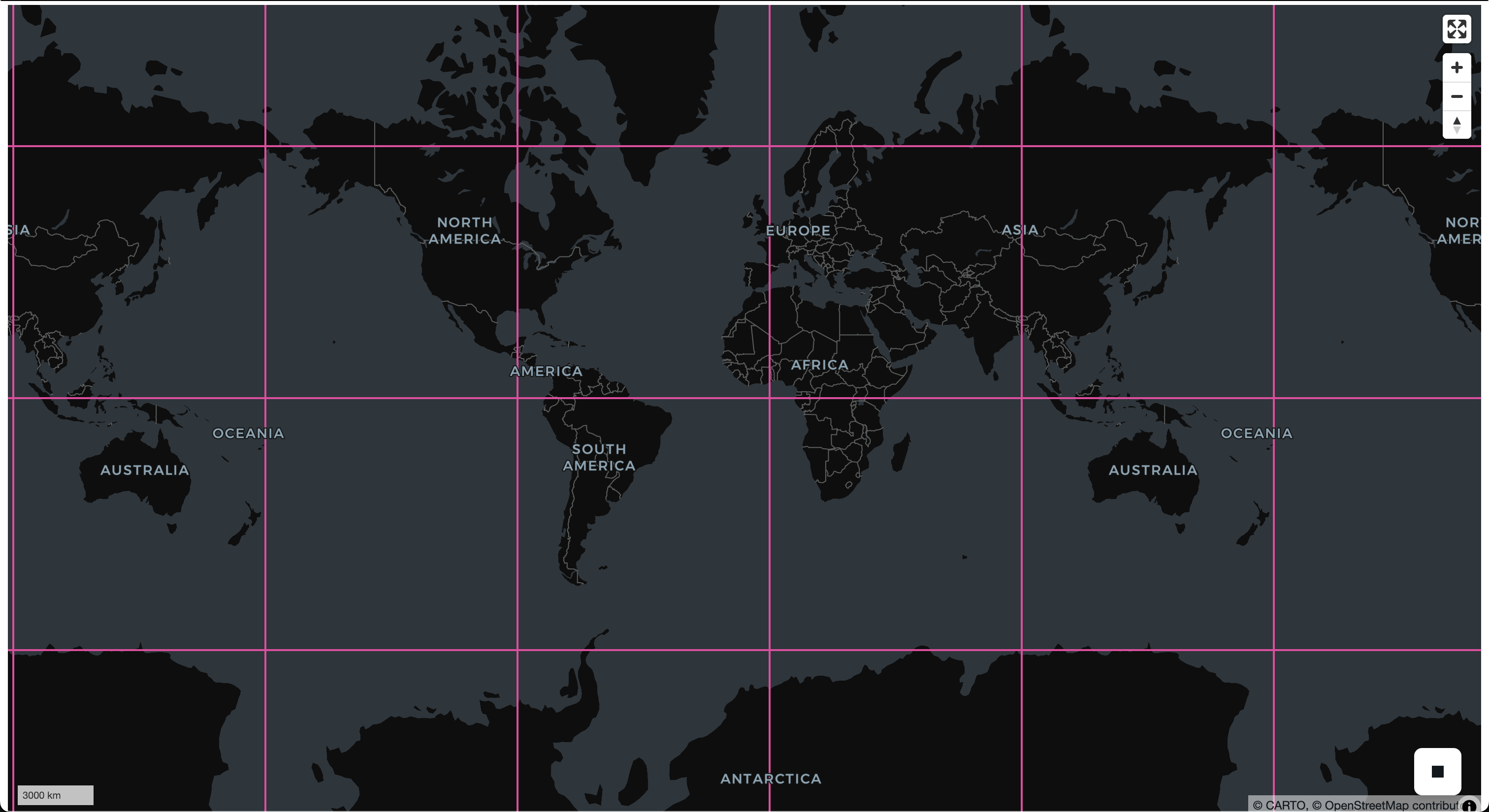
Because each year tiles into a 4 × 4 grid, the envelopes lay out that grid over the mapped extent — a picture of the cube's layout, drawn entirely from metadata. A LIMIT or row filter trims which chunks you draw (and, later, fetch).
Bring a plane into NumPy
A raster band carries its bytes, shape, and pixel type, so a materialized band decodes to a correctly-shaped, correctly-typed NumPy array in one call — Band.to_numpy():
planes = sliced.to_arrow_table()["plane"]
raster = planes[0].as_py()  # one 128x128 spatial tile for its year
band = raster.bands[0].to_numpy()
print(band.shape, band.dtype)
(128, 128) float32
Note that planes[0] currently forces a copy of the raster out of the Arrow buffer (a pyarrow limitation), so this path is not yet zero-copy. Rows correspond to chunks rather than a guaranteed order, so apply your own ordering (or carry a chunk identifier) if you need to know which tile and year a given plane covers.
Reading from cloud storage
The same code reads a datacube over S3 or HTTP(S) — only the URI changes. Supported schemes are file:// (and bare local paths), s3://, http://, and https://.
For S3, credentials come from the standard AWS environment variables (AWS_ACCESS_KEY_ID, AWS_SECRET_ACCESS_KEY, AWS_REGION). To read a public bucket anonymously, set the region and request unsigned access:
export AWS_REGION=us-west-2
export AWS_SKIP_SIGNATURE=true   # read public objects without credentials
# A real public bucket (CarbonPlan), readable with the settings above:
df = sd.read("s3://carbonplan-share/zarr-layer-examples/antarctic_era5.zarr")
Selecting arrays with the arrays option
By default SedonaDB discovers a group's arrays automatically — from the group's consolidated metadata when present, otherwise by listing the store. The arrays option names an explicit subset to read instead (as we did above):
spec = sedonadb_zarr.Zarr().with_options({"arrays": ["rain_ok"]})
df = sd.read(url, format=spec)
Naming arrays is needed in two situations:
- The store can't list and has no consolidated metadata. Plain HTTP servers generally can't list directories. Cloud Zarr groups often ship a consolidated-metadata block, so reads typically work without
arrays— but a group (or sub-group) lacking one can't be auto-discovered over such a store, and you must name the arrays. - The group mixes arrays with different shapes or chunk grids. Every array read together must share one chunk grid, so name a compatible subset (for example, read the data array and leave out a differently-shaped coordinate or CRS variable).
Because each row corresponds to one chunk, a LIMIT or row filter directly bounds how many chunks SedonaDB fetches — handy for sampling a large remote cube before committing to a full scan.