Rust Warps, SQL Calls, NumPy Reads: Three Rasters on One Grid

A satellite image and a land cover map of Seattle do not line up pixel for pixel. Each is a raster, a grid of pixels over the ground, and the grids differ: 10 m and 20 m pixels in the image, pixels measured in degrees in the map. Before any comparison, every pixel has to cover the same patch of ground in every file. SedonaDB 0.5.0, a database written in Rust, lines them up with two SQL functions. RS_Resample changes a raster's pixel size, and RS_ReprojectMatch moves a raster onto another raster's grid. NumPy then reads the three rasters as arrays of the same shape.

Why the pixels disagree

The image is one Sentinel-2 scene, S2C_10TET_20260807_0_L2A, from the public Sentinel-2 COGs bucket, with 0.0008 percent cloud. The map is the ESA WorldCover 2021 tile N45W123, the product of an earlier post. The scene counts in meters, in UTM zone 10. The tile counts in degrees of latitude and longitude. Over the same 60 m of ground in Seattle, the three grids look like this:

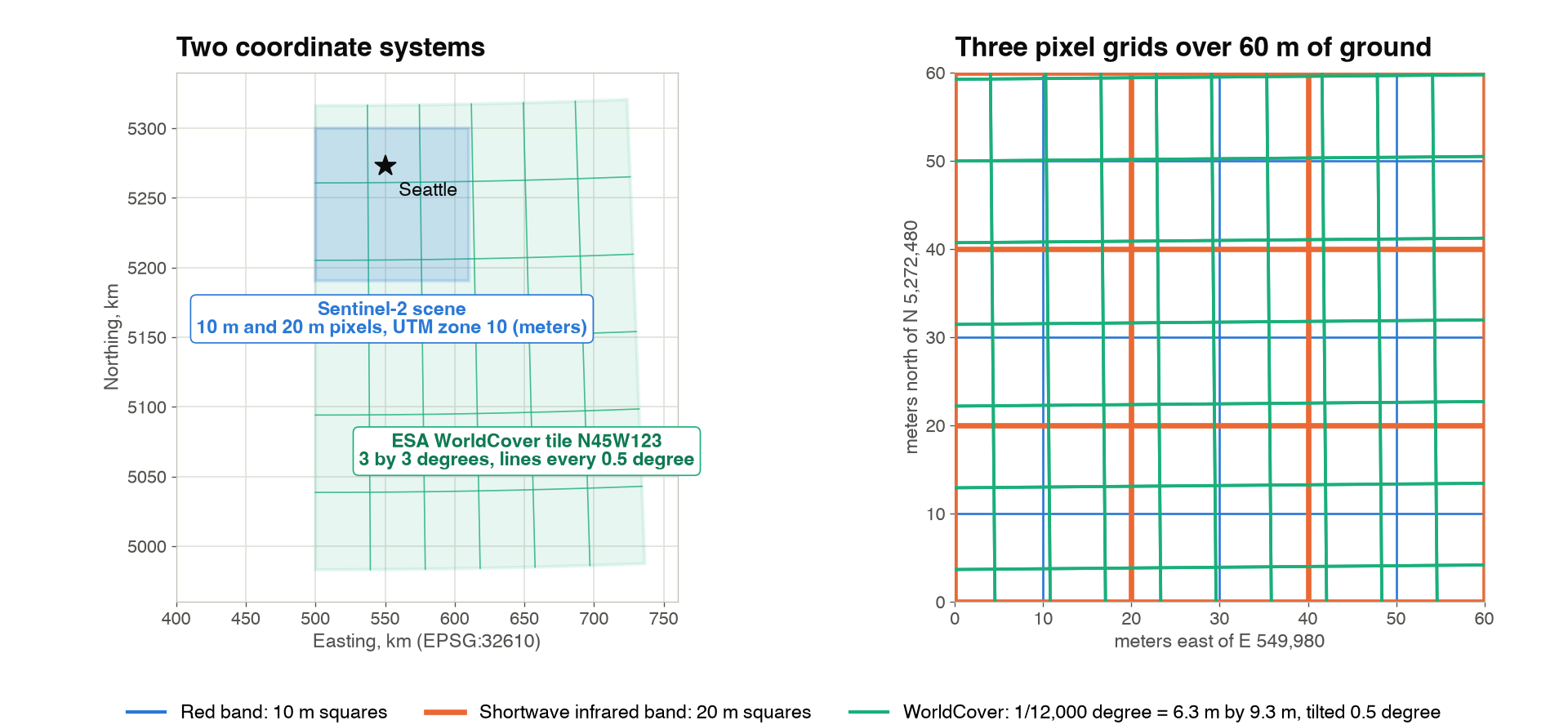
One shortwave infrared pixel holds four red pixels. One WorldCover cell is 6.3 m wide, 9.3 m tall, and tilted 0.5 degree from the scene's grid, because a step of 1/12,000 degree is shorter east to west than north to south at this latitude, and a line of constant longitude is not the scene's vertical. RS_FromPath reads the three headers over HTTPS:

import sedona.db
from sedonadb.raster import Raster

sd = sedona.db.connect()

SCENE = "https://sentinel-cogs.s3.us-west-2.amazonaws.com/sentinel-s2-l2a-cogs/10/T/ET/2026/8/S2C_10TET_20260807_0_L2A"
RED, NIR, SWIR = f"{SCENE}/B04.tif", f"{SCENE}/B08.tif", f"{SCENE}/B11.tif"
COVER = "https://esa-worldcover.s3.eu-central-1.amazonaws.com/v200/2021/map/ESA_WorldCover_10m_2021_v200_N45W123_Map.tif"

The query behind the table

sd.sql(f"""
    SELECT name, RS_FromPath(path) AS r
    FROM (VALUES ('red B04', '{RED}'), ('swir B11', '{SWIR}'), ('land cover', '{COVER}')) AS f(name, path)
""").to_view("rasters", overwrite=True)

sd.sql("""
    SELECT name, RS_Width(r) AS width, RS_Height(r) AS height, RS_SRID(r) AS srid,
           RS_ScaleX(r) AS pixel_size, RS_BandPixelType(r, 1) AS pixel_type
    FROM rasters
""").show()

┌────────────┬───────┬────────┬────────┬────────────────────────┬─────────────────┐
│    name    ┆ width ┆ height ┆  srid  ┆       pixel_size       ┆    pixel_type   │
╞════════════╪═══════╪════════╪════════╪════════════════════════╪═════════════════╡
│ red B04    ┆ 10980 ┆  10980 ┆  32610 ┆                   10.0 ┆ UNSIGNED_16BITS │
│ swir B11   ┆  5490 ┆   5490 ┆  32610 ┆                   20.0 ┆ UNSIGNED_16BITS │
│ land cover ┆ 36000 ┆  36000 ┆   4326 ┆ 0.00008333333333333333 ┆ UNSIGNED_8BITS  │
└────────────┴───────┴────────┴────────┴────────────────────────┴─────────────────┘

Same CRS, different pixel size

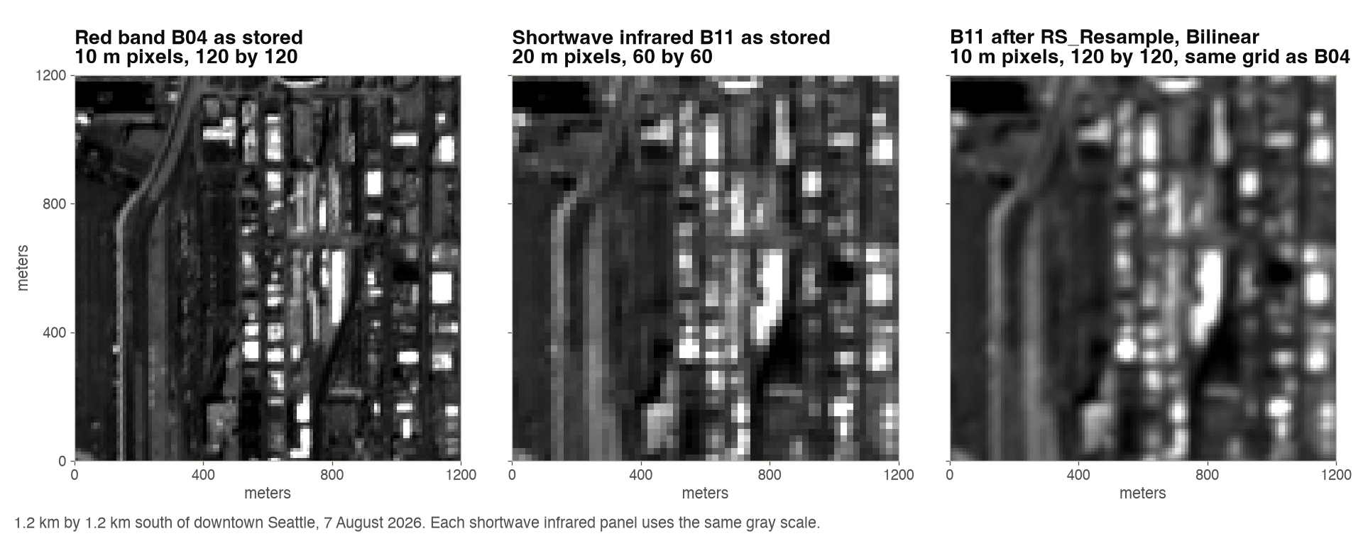
The shortwave infrared band shares the red band's coordinate system, so only the pixel size has to change. RS_Resample takes the red band as its reference and returns the shortwave infrared band with the same 10,980 by 10,980 grid:

swir_tbl = sd.sql(f"""
    SELECT RS_Resample(RS_FromPath('{SWIR}'), RS_FromPath('{RED}'), false, 'Bilinear') AS r
""").to_arrow_table()
swir = Raster(swir_tbl["r"], 0).to_numpy()[0]  # (10980, 10980) uint16

Bilinear gives each 10 m pixel a weighted mix of the four nearest 20 m values, the right choice for a measurement. The false says the reference supplies a pixel count; true would make it supply a pixel size.

Different CRS

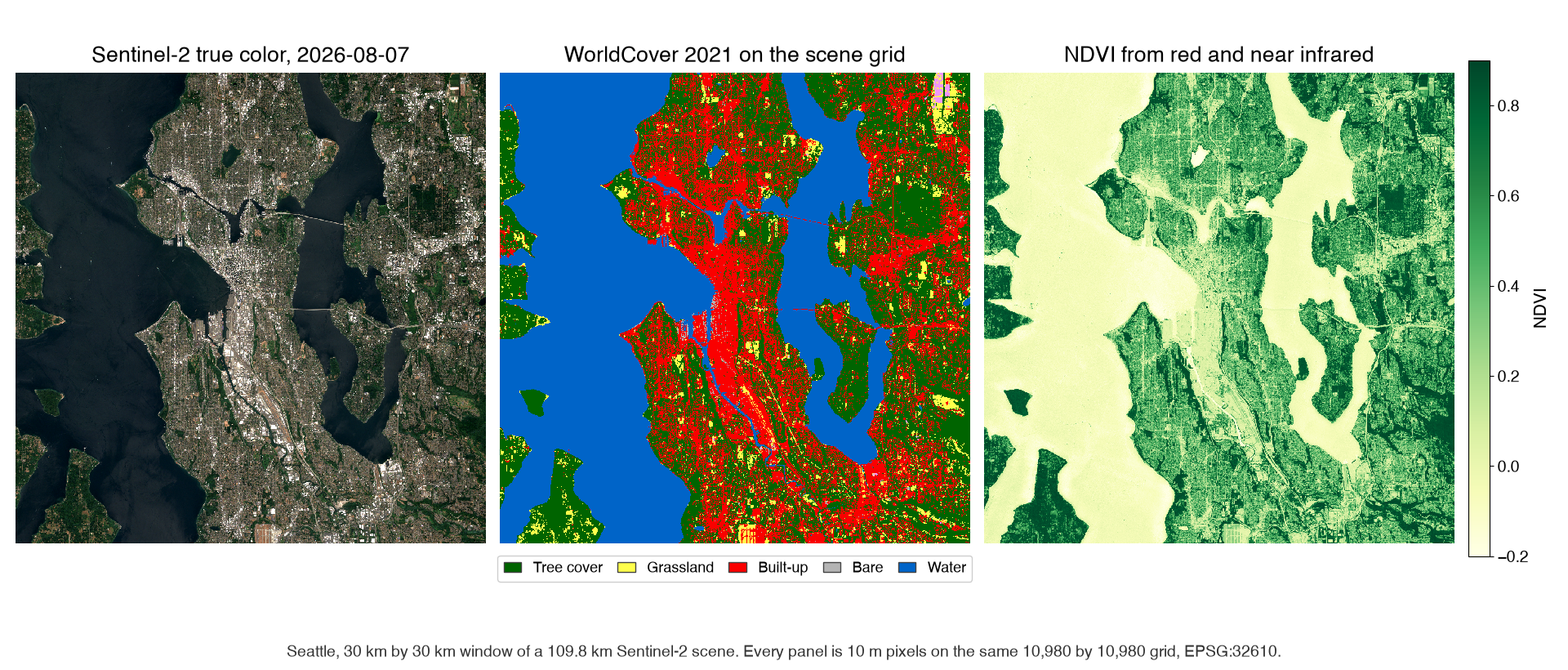
The land cover map is in degrees. RS_ReprojectMatch moves it onto the red band's grid: same coordinate system, same extent, same pixel size, same width and height. The reference contributes only its grid, and its pixels are never read. SedonaDB, written in Rust, calls GDAL's warp for the pixel math.

sd.sql(f"""
    SELECT RS_ReprojectMatch(RS_FromPath('{COVER}'), RS_FromPath('{RED}'), 'NearestNeighbor') AS r
""").to_memtable().to_view("cover_on_grid", overwrite=True)

The algorithm is NearestNeighbor because the values are class codes. Code 10 is tree cover and code 50 is built-up land; their average, 30, is grassland, and no pixel in Seattle became grassland by being half tree and half roof. to_memtable keeps the result in memory, so later queries read the aligned map without computing it again.

NumPy does the rest

All three rasters now share one grid, so an array index means the same patch of ground in each. to_numpy returns each band as a NumPy array, and the normalized difference vegetation index (NDVI), which compares near infrared and red, groups by land cover code with np.bincount:

NDVI per land cover class

import numpy as np


def band(path):
    tbl = sd.sql(f"SELECT RS_EnsureLoaded(RS_FromPath('{path}')) AS r").to_arrow_table()
    return Raster(tbl["r"], 0).to_numpy()[0]


red, nir = band(RED), band(NIR)
cover = Raster(
    sd.sql("SELECT r FROM cover_on_grid").to_arrow_table()["r"], 0
).to_numpy()[0]

valid = (red > 0) & (nir > 0) & (swir > 0) & (cover > 0)
r, n = red.astype(np.float32), nir.astype(np.float32)
with np.errstate(invalid="ignore", divide="ignore"):
    ndvi = (n - r) / (n + r)

c = cover[valid]
count = np.bincount(c, minlength=101)
mean_ndvi = np.bincount(c, weights=ndvi[valid], minlength=101) / np.maximum(count, 1)

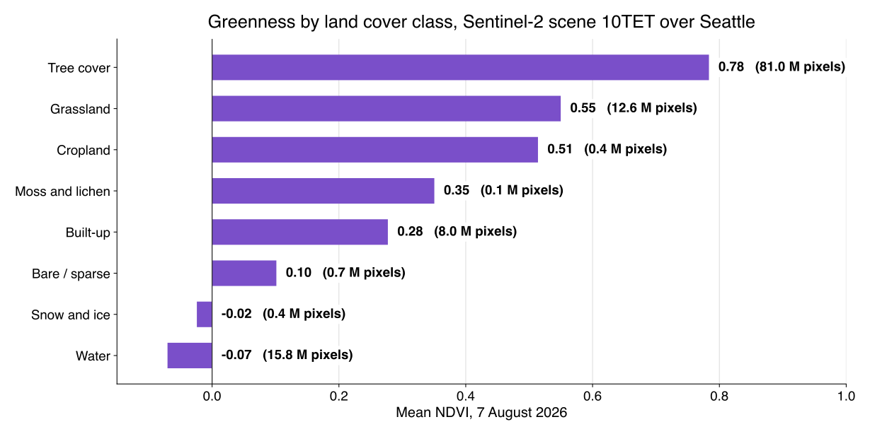
Tree cover is 68 percent of the 119 million valid pixels and averages an NDVI of 0.78. Built-up land averages 0.28, and water is below zero. The same arrays give the moisture index from the shortwave infrared band, where snow on the Cascade peaks scores highest of any class, 0.50.

Mode or NearestNeighbor

Both functions accept seven algorithms: NearestNeighbor, Bilinear, Cubic, CubicSpline, Lanczos, Average, and Mode. Measurements take a weighted mix. Class codes take NearestNeighbor, the code under the new pixel's center, or Mode, the code that covers most of the new pixel. One query each turns the aligned map into a 100 m map:

sd.sql("SELECT RS_Resample(r, 1098, 1098, false, 'Mode') AS r FROM cover_on_grid")

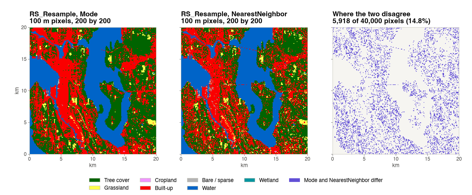
Over the whole scene the two maps disagree on 6.83 percent of the 100 m pixels, and in the 20 km window above on 14.8 percent. Where they disagree, Mode says tree cover more than twice as often as NearestNeighbor, because a 100 m square in Seattle is often mostly trees with one road or roof under its center. Both queries together took 0.29 seconds from the in-memory view.

The point

• RS_Resample changes the pixel size inside one coordinate system. RS_ReprojectMatch moves a raster onto another raster's grid, coordinate system included. Name a reference raster and the output has its width, height, origin and CRS.
• The algorithm is a statement about the data: Bilinear for measurements, NearestNeighbor or Mode for classes.
• Once the grids match, SQL and NumPy share the same pixels. The whole script, every file read over HTTPS, ran in 73 seconds on one machine.

Both functions are marked experimental in the 0.5.0 reference, so their signatures may still change. The SedonaDB raster introduction used RS_ReprojectMatch to average eleven PlanetScope scenes onto one grid, and the 0.5.0 release post lists the other raster functions that arrived with it.

Sentinel-2 L2A scene S2C_10TET_20260807_0_L2A from the Sentinel-2 COGs bucket; contains modified Copernicus Sentinel data (2026). Land cover from ESA WorldCover 2021 v200, CC BY 4.0; contains modified Copernicus Sentinel data (2021) processed by the ESA WorldCover consortium. Measurements on SedonaDB 0.5.0, one machine with 10 cores. SedonaDB reference: RS_Resample, RS_ReprojectMatch, RS_FromPath.

Star Apache Sedona on GitHub

A star takes two seconds and helps others discover the projects.

apache/sedona apache/sedona-db apache/sedona-spatialbench